Parameters: Transient Solver

Description

Dynamic simulations are performed on systems with one or more degrees of freedom. The dynamic simulation accounts for all inertia effects, all applied forces, and internal constraints. This enables you to run accurate system level simulations of complex mechanical systems.

Format

<Param_Transient
 [ integrator_type = "string" ]
 [ integr_tol = "real" ]
 [ h_max = "real" ]
 [ h_min = "real" ]
 [ h0_max = "real" ]
 [ vel_tol_factor = "real" ]
 [ rel_abs_tol_ratio = "real" ]
 [ max_order = "integer"]
 [ dae_alg_tol_factor = "real" ]
 [ dae_index = "integer"]
 [ dae_constr_tol = "real" ]
 [ dae_corrector_maxit = "real" ]
 [ dae_corrector_minit = "real" ]
 [ dae_vel_ctrl = "TRUE|FALSE" ]
 [ dae_jacob_eval = "integer" ]
 [ dae_eval_expiry = "integer" ]
 [ dae_jacob_init = "integer" ]
 [ dae_interpolation = "TRUE|FALSE" ]
 [ newmark_beta = "real" ]
 [ newmark_gamma = "real" ]
 [ hht_alpha = "real" ]
/>

Attributes

integrator_type

Defines the integrator to be used with the ODE form of the equations of motion. Select one of the following:

Integrator	Family	Form of Equations (see Comment 3)	Integration Method (see Comment 1)	Feature	Max Order
DSTIFF	DASPK (Large Scale Differential Algebraic Equation Solver)	DAE	implicit	Variable step and order	5
CSTIFF	DASPK	DAE	implicit	Fixed step and order	5
NSTIFF	Newmark	DAE	implicit	Variable step and fixed order	1
HSTIFF	HHT (Hilber-Hughes-Taylor)	DAE	implicit	Variable step and fixed order	2
VSTIFF	VODE (Variable-Coefficient Ordinary Differential Equation)	ODE	implicit	Variable step and order	5
MSTIFF	MEBDF (Modified Extended Backward Differentiation Formulae)	ODE	implicit	Variable step and order	9
ABAM	ABAM (Adams-Bashforth-Adams-Moulton)	ODE	explicit	Variable step and order	12

The default value for integrator_type is DSTIFF. It is the default integrator in MotionSolve due to its maturity, stability, and applicability to a wide range of models. See the Comments below for references to each of these integrators.

integr_tol

Represents the maximum absolute error per step that the integrator is allowed in computing the displacement, velocity, and differential equations states.

Since displacement and velocity have different units, they are subject to different error tolerances.

• Displacement tolerance = integr_tol
• Velocity tolerance = vel_tol_factor*integr_tol
• Differential equation state tolerance = integr_tol
• Algebraic state tolerance = dae_alg_tol_factor *integr_tol (DAE only)

The default value for integr_tol is 1.0E-3.

vel_tol_factor is a scale factor that you specify separately.

If integrator type is CSTIFF, this attribute is used for monitoring purposes only. MotionSolve provides a message whenever the measured error is greater than any of the above-mentioned tolerances.

h_max

Defines the maximum step size the integrator is allowed to take. You can also use this parameter to control the accuracy of the results. Generally, a smaller time step leads to more accurate results. For models with discontinuities, such as contact, a smaller value of h_max should be specified.

The default value for h_max is 1.0E-3.

If integrator type is CSTIFF, then h_max defines the fixed step.

Note: The maximum integrator step size is set to the print_interval in the Simulate command if the print_interval is smaller than h_max.

h_min

Defines the minimum step size the integrator is allowed to take.

The default value for h_min is 1.0E-6.

If integrator type is CSTIFF, this attribute is ignored.

h0_max

The maximum initial step size.

The default value for h0_max is 1.0E-8.

If integrator type is CSTIFF, this attribute is ignored.

vel_tol_factor

A factor that multiplies integr_tol to yield the error tolerance for velocity states.

The default value for vel_tol_factor is 1000. A good value for vel_tol_factor can generally be calculated as 1/h, where h is the dominant step size for your simulation. To try and reduce the analysis time, a value larger than the default 1000 may be used. However, this will reduce accuracy in the velocity states of your model.

rel_abs_tol_ratio

The factor that multiplies integr_tol to yield the relative error tolerance for the integrator.

The default value is 0.01.

If integrator type is CSTIFF, this attribute is used for monitoring purposes only. MotionSolve provides a message whenever the measured error is greater than the relative error tolerance.

max_order

Specifies the maximum order that the integrator is to take. Each integrator has its own built-in maximum order. Higher orders lead to higher accuracy, but lower stability in the numerical method. The table above shows the maximum order for the various integrators in MotionSolve. For models that contain contact or other discontinuous events, it may be beneficial to set max_order = 2.

If integrator type is CSTIFF, then max_order defines the fixed order.

Attributes (specific to DAE solvers)

dae_alg_tol_factor

The factor that multiplies integr_tol to yield the error tolerance for algebraic states like Lagrange Multipliers.

The default value for dae_alg_tol_factor is 1000.

dae_index

The index of the DAE formulation.

Index 3 indicates that position constraints are added to the equations of motion.

Index 1 indicates that position, velocity, and acceleration constraints are added (Stabilized Index 1).

See Comments 3-4 for more detailed information.

The default value for dae_index is 3.

dae_constr_tol

The tolerance on all algebraic constraint equations that the corrector must satisfy at convergence.

The default value for dae_constr_tol is 1.0E-5. Decrease this value only if you see a lot of "noise" in the joint or motion reaction forces. Smaller values for this attribute will decrease the speed of the solution. 11

If integrator type is CSTIFF, this attribute is used for monitoring purposes only. MotionSolve provides a message whenever the measured error is greater than the algebraic constraint tolerance.

dae_corrector_maxit

The maximum number of iterations that the corrector is allowed to take to achieve convergence.

The default value for dae_corrector_maxit is 4. Under no circumstances should this be increased beyond 8. If the results don't converge for a particular time step, it may be better to let the integrator fail and try to solve with a smaller time step.

If integrator type is CSTIFF, then dae_corrector_maxit defines the fixed number of iterations within each time step.

dae_corrector_minit

The minimum number of iterations that the corrector is allowed to take before it checks for corrector divergence.

The default value for dae_corrector_minit is 0. A value of 0 lets the integrator choose the minimum number of iterations. The integrator may choose to skip corrector iterations if the norm is less than the tolerance for a given step.

Under no circumstances should this be increased beyond 3.

If integrator type is CSTIFF, this attribute is ignored.

dae_vel_ctrl

The logical flag that controls whether the velocity states are checked for local integration error at each step. This is only valid for the SI1 integrator (see dae_index).

• "TRUE" indicates that the integrator is to include velocity states in its check for local integration at the end of each step.
• "FALSE" indicates that the integrator is to exclude velocity states in its check for local integration at the end of each step.

When not specified, this defaults to "TRUE" for the SI1 formulation and "FALSE" for the I3 formulation. For more information on formulations, refer to comments 5-6.

Integrator

DAE_VEL_CTRL

I3 Formulation

"FALSE"

SI1 Formulation

"TRUE"

The I3 formulation is not designed to track velocity errors. Hence, even when DAE_VEL_CTRL is "TRUE" for I3, velocity errors will not be tracked.

dae_jacob_eval

This attribute controls the frequency of evaluation of the Jacobian matrix during corrector iterations.

0

Implies that the integrator automatically determines when a new Jacobian is needed by examining the rate of convergence.

1

Implies that a new Jacobian is to be calculated at every iteration.

2

Implies that a new Jacobian is to be calculated at every other iteration, for example at iteration 1-3-5, and so on.

3

Implies that a new Jacobian is to be calculated at every third iteration, for example at iterations 1-4-7, and so on.

Specify dae_jacob_eval only when the default setting does not work well. Frequent Jacobian iterations can slow down the simulations dramatically.

When not specified, the integrator automatically determines when a new Jacobian is needed by examining the rate of convergence.

The Jacobian evaluation is also affected by the attribute dae_jacob_init. 12

If integrator type is CSTIFF, then dae_jacob_eval needs to be greater or equal to 1.

dae_eval_expiry

This is an optional attribute. It defines the number of integration steps after which the evaluation pattern defined by dae_jacob_eval is ignored, and the default evaluation pattern is to be used. The default evaluation pattern is automatically determined when a new Jacobian is needed by examining the convergence rate of the corrector.

For example, dae_eval_expiry = "10" indicates that after 10 successful integration steps, the pattern specified by dae_jacob_eval is to be ignored.

The default value of dae_eval_expiry is 0, which means that the pattern specified by dae_jacob_eval is obeyed throughout the simulation.

Use this flag when you want dae_jacob_eval to be in effect only to overcome an initial transience in the system.

If integrator type is CSTIFF, this attribute is ignored.

dae_jacob_init

This attribute specifies the number of initial Jacobian matrix evaluations during corrector iteration.

0

Implies that the integrator automatically determines when a new Jacobian is needed by examining the rate of convergence.

1

Implies that a new Jacobian is to be calculated at the first iteration and none afterward.

2

Implies that a new Jacobian is to be calculated at the first and second iterations, none afterward, as so on with higher values of this setting.

Default = 0

If integrator type is CSTIFF, then dae_jacob_init needs to be greater or equal to 1.

dae_interpolation

Specifies whether the integrator uses interpolation for the results at the output steps.

• TRUE means that MotionSolve interpolates (as needed) the results at the output points requested by the user.
• FALSE means that MotionSolve uses the DASPK integrator to interpolate (as needed) the results at the output points requested by the user.

Default = TRUE

If integrator type is CSTIFF, this attribute is ignored.

newmark_beta

Specifies the beta coefficient in the Newmark-beta method. See references in the comments to learn more about the coefficient.

Default = 0.36.

This attribute is used only if integrator type is NSTIFF.

newmark_gamma

Specifies the gamma coefficient in the Newmark-beta method. See references in the Comments to learn more about the coefficient.

Default = 0.7.

This attribute is used only if integrator type is NSTIFF.

hht_alpha

Specifies the alpha coefficient in the Hilber-Hughes-Taylor method. Beta and gamma coefficients are derived from the alpha coefficient. See references in the Comments to learn more about these coefficients.

Default = 0.33.

This attribute is used only if integrator type is HSTIFF.

Comments

1. Explicit vs Implicit Integration Methods

   Explicit and implicit integration are numerical methods for obtaining approximations to the solution of time-dependent equations. Explicit integrators calculate the state of a system at t_n+1 from the state at t_n. This calculation can be done explicitly in one step. Implicit integrators find a solution by solving an equation involving states from both times, t_n+1 and t_n. The latter requires an iterative process to find the solution and, hence, can be computationally more expensive at each time step. They can also introduce some numerical damping into the system that might or might not be desired, depending on the application. However, implicit integrators usually allow for larger step size Δt = t_n+1 – t_n, and are better suited for numerical stiff equations (see Comment 2), and can solve differential algebraic equations (see Comment 3).

2. Numerical and Physical Stiffness

   Numerical stiffness is quite different from "physical" stiffness. Numerical stiffness is governed by the damping characteristics of a system, whereas physical stiffness is governed by the stiffness intrinsic to the system (for example, a spring in the system). The concept of numerical stiffness is quite closely related to the eigenvalues of the system at an operating point.

   The eigenvalues of a system have two components: the real part and the imaginary part. The real part defines the damping characteristics of the system, and the imaginary part defines the vibration frequencies of the system at the operating point.

   • An eigenvalue with no imaginary component defines an over-damped vibration mode.
   • An eigenvalue that has no real component defines an undamped vibration mode.
   • A complex eigenvalue defines an under-damped vibration mode.
   A numerically stiff system is characterized by widely separated eigenvalues that exhibit the following properties:

   • The high frequency components are over-damped and rapidly decay.
   • The low frequency components of the solution exhibit under-damped behavior.

   The concept of numerical stiffness is explained using the simple example shown below.

   The figure below depicts two unconnected spring-mass systems. The first system has a mass M₁ supported by a spring with properties K₁, C₁ and L₀₁. The second system has a mass M₂ supported by a spring with properties K₂, C₂ and L₀₂. The displacement of mass M₁, measured with respect to a global coordinate system, is denoted as x₁. The displacement of mass M₂, measured with respect to a global coordinate system, is denoted as x₂.

   Assume:

   • M1=1Kg, C1=2 N sec/m and K1=10⁴ N/m
   • M2=1Kg, C2=2x104 N sec/m and K2=10⁸ N/m

   
   
   Figure 1. Two Unconnected, Simple Spring-mass Systems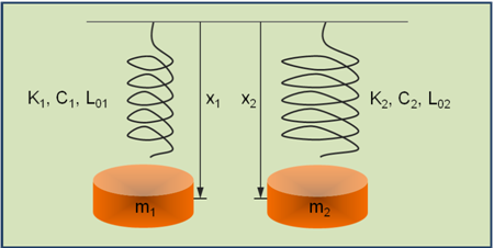

   For each system, i, the following are easily ascertained:

   • The equation of motion for system-i is:
     (1)

     $$M_i{\ddot{x}}_i+C_i{\dot{x}}_i+K_i\left(x_i-L_{0i}\right)=0$$
   • The eigenvalues for system-i are:
     (2)

     $${\lambda }_i=\frac{-C_i\pm \sqrt{C_i^2-4K_i{M}_i}}{2M_i}$$
   • The eigenvalues and response for the first system is:
     (3)

     $$\begin{array}{l}{\lambda }_1=-1\pm 99.995i\\ x_1(t)=X_{01}{e}^{-(1\pm 99.995i)t}=X_{01}{e}^{-t}\left[\cos \left(99.995t\right)+i\cdot \sin \left(99.995t\right)\right]\end{array}$$
   • The eigenvalues and response for the second system is:
     (4)
     
     

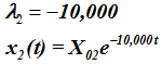
     System 1 is under-damped. It will display decaying oscillations in response to an initial disturbance. After 0.01 seconds, the initial disturbance is reduced by a factor = e^-0.01 = 0.99 of the original value. System 1 oscillates at a frequency of 99.995 radians/sec.

     In contrast, system 2 is over-damped. After 0.01 seconds, the initial disturbance is reduced by a factor = e^-100 = 3.72 x 10^-44 of the original value. For any initial disturbance, system response is almost instantaneously damped out. System 2 does not oscillate at all.

     A system exhibiting these characteristics is called numerically stiff. One component of the solution exhibits slow decay to an initial excitation whereas another component rapidly dies almost instantaneously.

     Many mechanical systems have numerically stiff properties or are characterized by differential-algebraic equations (see Comment 3). In general, these can only be solved efficiently using an implicit integration method.

3. Differential Algebraic Equations
   A system of equations, which is a combination of ordinary differential equations (ODE), and algebraic constraint equations are called differential algebraic equations (DAE).

   
   
   Figure 2. A Multibody system.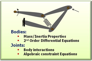

   For example, in a multibody system (MBS), Newton's second law manifests itself in the form of second order, ordinary differential equations (ODE) while constraints in the system (joints, for example) manifest themselves as algebraic equations (AE). Hence, the mathematical representation of a typical multibody system is a system of differential algebraic equations (DAE). The mechanism shown in the figure above is usually characterized by differential algebraic equations.

   Ordinary differential equations are represented as: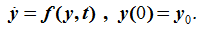(5)
   
   

   y are the states to be integrated.

   Differential algebraic equations are represented as: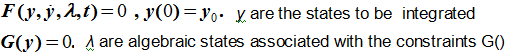(6)
   
   
4. Index of a DAE
   The index of a system of DAEs is defined as the number of times you need to differentiate the constraints in the system with respect to the independent variable (usually time), to get a system of ordinary differential equations. This is illustrated in the figure below.

   
   
   Figure 3. Index of a system of DAEs.

5. Equation Formulation
   MotionSolve supports three different equation formulations for dynamic simulations:

   The ODE formulation

   The ODE formulation supports both stiff and non-stiff integrators. MotionSolve transforms the DAE form equations of motion into ODE form equations using coordinate partitioning and then solves the resulting equation using an ODE integrator. Both stiff and non-stiff integrators are supported. The stiff integrators supported by this formulation are (a) VSTIFF and (b) MSTIFF. The integrator ABAM is used to integrate non-stiff solutions.

   The DAE Index-3 (I3) formulation

   The I3 formulation provides the DAE form of the equations of motion to an integrator capable of solving this form of the equations of motion. DSTIFF, CSTIFF, NSTIFF, and HSTIFF are capable of solving the I3 form of the equations of motion. In the I3 formulation, the integrator does not monitor the integration local error in the velocity states. Consequently, I3 solutions typically tend to be very fast, though slightly inaccurate in velocities sometimes.

   The DAE Stabilized Index-1 (SI1) formulation

   The SI1 formulation provides an even more "stabilized" index-1 DAE form of the equations of motion to an integrator capable of solving this form of the equations of motion. The term "stabilized" refers to the seemingly redundant set of velocity and acceleration constraints that are added to the I3 set. These enforce consistency of velocities and accelerations with the velocity and acceleration constraints - which would be automatic if the solutions were exact. DSTIFF, CSTIFF, NSTIFF, and HSTIFF can solve the SI1 form of the equations of motion. In the SI1 formulation, the integrator monitors the integration local error in both the displacement and velocity states. Consequently, SI1 solutions typically tend to be very accurate. The typical speed of SI1 solutions, compared to I3 solutions, is somewhat slower.

6. Index-3 DAE form of the Equations of Motion
   Assume that a system is defined as follows:

   • "N" displacement coordinates q=[q1, q2, … qN]^T are used to represent the system.
   • The coordinates q are not all independent.
   • "M" displacement constraints Φ =[ Φ1(q,t), Φ2(q,t), … ΦM(q,t)]^T exist between the "N" coordinates q.
   • Let λ = [ λ1, λ2 … λM]^T represent Lagrange Multipliers required to maintain the constraints Φ.
   • Let F = [F1, F2 … FNa]^T represent external forces acting on the system.
   • Let the kinetic energy of the system be and the potential energy be.
   • Then the Lagrangian function may be expressed as .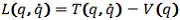
     Under these assumptions, the equations of motion for the system can be represented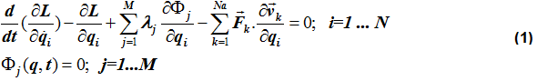
     
     as:
   The above equations are called the Euler-Lagrange representation of the equations of motion. In matrix form, equation (1) can be written as:
   
   

   Equations (2.1) represent the force balance equations. The first term represents the inertia force, the second term represents the constraint forces and the third term the generalized external forces. Equations (2.1) are thus a restatement of Newton's Second Law of Motion. Equations (2.1) are a differential equation that relates the time derivative of velocity (acceleration) to the external and internal forces acting on the system.

   Equations (2.2) represent the kinematic differential equations in the system. These equations represent the equations of motion in first order form. To accomplish this, a new set of variables, u, the velocities are created. Velocities are defined as first-time derivatives of displacements. Equations (2.2) are also differential equations.

   Equations (2.3) represent the algebraic constraints in the system. These come into existence because the equations were not formulated in terms of an independent coordinate set. The system has p=N-M degrees of freedom. The N coordinates therefore can be related to each other through M algebraic constraint equations.

   Equations (2.4) represent the user-defined differential equations, specified using Control_Diff, Control_SISO, and Control_StateEqn elements. The user-defined states are denoted by x.

   Equations (2) are a set of implicit, differential-algebraic equations (DAE). Let Z = [u, q, λ, x]^T. Equations (2) can be represented in compressed notation as:
   
   
   By differentiating equations (2.1) once and equations (2.3) three times, you can convert equations (3) to a set of Ordinary Differential Equations (ODE) of the form:
   
   
   The index of a DAE is defined as the number of times the constraints are to be differentiated in order to convert the DAE to a set of ODE. Since three time differentiations of the constraints (2.3) are needed to arrive at the ODE form represented by equations (4), the index of the DAE is said to be 3. Index-3 DAE are also characterized by the fact that the matrix
   
   

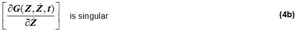
   A numerical solution of equations (2) or (3) requires specialized DAE integrators. These methods share the basic concept that accuracies in {u}, {q} and {λ} are controlled to different levels. One common approach (Index-3) is to ignore local integration error in {u} and {λ} and monitor local integration error in {q} only. Index-3 solutions thus tend to be less accurate, but very fast. If extremely accurate solutions are required, an alternative approach for the solution is preferred.

7. Numerical Integration of the Equations of Motion Using Implicit Integrators
   Each implicit integrator must perform three key operations for each time step:

   1. Predict
      The purpose of the predictor is to provide a good initial guess for the corrector. The predictor fits a polynomial through the previously calculated solution points. It then extrapolates the polynomial to the new value of time to "predict" the solution, as shown below.

      
      
      Figure 4. The Predictor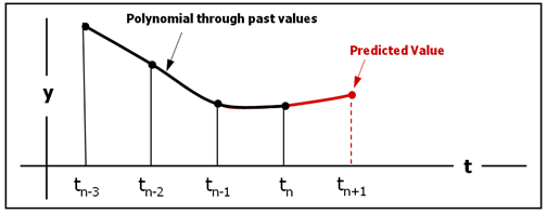

   2. Correct

      The purpose of the corrector is to refine the prediction iteratively until it satisfies the equations of motion. This iterative refinement process often involves the use of methods such as the Newton-Raphson method.

   3. Estimate local truncation error

      The corrector's primary role is to enforce that the solution satisfies the equations of motion, but it doesn't guarantee overall accuracy. Subsequently, the next step in the process involves calculating the integration error within the step to estimate accuracy. This is necessary because the corrected solution may not necessarily represent the "true" solution. For example, if the initial prediction is too far off the true solution, the corrector may have converged to a solution that no longer aligns with the model's initial conditions. In essence, your result may have transitioned to a different solution within the solution manifold, albeit one that still adheres to the equations of motion.

8. My model fails due to integrator failures. How can I diagnose this issue and fix it?

   Multi-step integrators, like DSTIFF and others, estimate the local error at each step by computing the difference between the predicted and the corrected value of the solution, and scaling it by an "error coefficient" that is calculated by the integrator. A bad prediction can therefore cause an integration error.

   Predictions can be inaccurate for two reasons:

   • There is a discontinuous motion input in the system.
   • There is an almost discontinuous force in the system.
   The effect of such modeling is shown below.

   
   
   Figure 5. Discontinuities are the root cause of integration failures.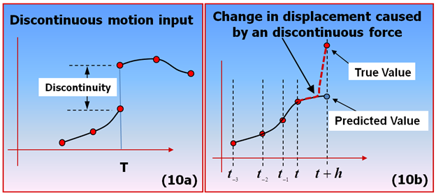

   Discontinuities such as those shown above can be caused by function expressions or user subroutines that use IF-THEN-ELSE logic carelessly. Modeling elements that should be examined for discontinuities or sharp changes include:

   • Forces
   • Variables
   • User Differential Equations
   • General State Equations

   It is a good idea to replace IF-THEN-ELSE logic with smooth STEP functions.

   Also, use the MotionSolve XML statement:

   <DebugOutput>
         SwitchOn="True"
   </DebugOutput>

   to enable detailed Newton-Raphson iteration output. By looking at this output, you can usually backtrack to the modeling elements that are likely causing the failure.
   The standard approach for addressing typical integration issues includes the following steps:

   • Ensure that stiffness and damping coefficients are set to realistic values.
   • Verify that masses and inertias are assigned values that are physically meaningful.
   • Identify and rectify any discontinuities in the modeling elements.
   • Exercise caution with very steep step functions.
   • As a temporary measure, consider relaxing the integration tolerance (INTEGR_TOL) to better understand the underlying issue.
9. Have my results converged? That is, have they stopped changing with the error tolerance?
   It's recommended that you perform a convergence study to ensure that the results you get from the integrator have stopped changing (are converged). Since the integrator is approximating an exact solution, it is possible that allowing too much error in the integrator causes the integrator to provide a different result than if the error tolerance is tighter (smaller). There are a range of settings to allow you to tune the integrator as desired, but the few to start investigating first are the following:

   • integr_tol
   • h_max
   • vel_tol_factor for DSTIFF, which requires SI1 and via the dae_index parameter
   You may get converged results in different ways, but below is one example that may work for you:

   • Pick the channels of data you are interested in the model (displacements, forces, and so on).
   • Pick the integrator - what does it perform error control on? (displacements, velocities, differential states).
   • Reduce the error until the states that the integrator controls converge. Then, take the largest error that gives the converged result.
   • If you're still interested in the states that the integrator does not control with error tolerance, reduce the integrator maximum step size (h_max) until those states converge. Then, use the largest h_max that gives the converged results.
   • If the simulation fails, you can loosen (increase) error tolerance and control accuracy with the integrator maximum step size (h_max) to try to get past the problem. This will likely take more time than for a variable-step integrator, so use as a last resort.
   • Many other integrator settings are also available, so consider exploring other options that may be applicable to your model.
10. Relative Comparison of the Various Formulation Approaches
    The table below summarizes the relative strengths of the different DAE approaches. The following criteria are used to characterize the different approaches:

    Accuracy

    Measures the integration error that is accumulated in the solution array.

    Speed

    Measures the relative CPU time commonly seen for the different approaches. This is highly model-dependent, and reflects our experiences to date in testing the various approaches.

    Handling Discontinuities

    Measures the ability of the formulation to deal with a sharp corner or a discontinuity in a system input (Motion or Force). Discontinuities and sharp corners (non-differentiability) should be avoided in models.

    Consistency

    Measures how well the solution satisfies the constraints Φ and its first and second time derivatives.

    Tracking High Frequencies

    Measures how well high frequencies in a system are tracked.

    Numerical Damping

    Measures the numerical damping applied because of the implementation of a certain index formulation. In general, high numerical damping leads to faster and more robust solutions, though at the expense of some accuracy.

    Robustness

    The default DAE formulation is Index-3. We recommend that you use the Index-3 formulation first, and consider switching to other formulations only if a solution is found that lacks in the criteria shown above.

    Note: The table below contains subjective information, and should therefore be regarded as a general guideline, not an absolute recommendation.

    Table 1. Relative merits of the different equation formulations.

    	I-3	SI-1	ODE (SI-0)	ABAM
    Accuracy	Medium	High	High	High
    Speed	High	Medium	Low	High / Very Low*
    Handling Discontinuities	High	Low	Low	High
    Consistency	Low	High	High	High
    Tracking High Frequencies	Low	High	High	High
    Numerical Damping	High	Low	Low	Low
    Robustness	High	Medium	Medium	High

    (*For ABAM, Speed is high for non-stiff and very low for stiff problems.)
11. Increasing DAE_CONSTR_TOL above 0.001 mm is generally not advisable. This tolerance governs the minimum solution accuracy for the kinematic constraints in the system specified in the length units of the model. When DAE_CONSTR_TOL is large (greater than 0.001 mm), the system constraints can be only loosely satisfied. In addition to creating inaccurate answers, errors in constraint satisfaction can also cause the numerical solution to become unstable and even cause failures.
12. The dae_jacob_eval and dae_jacob_init both control when the Jacobian is evaluated during the corrector iterations. The key difference between the two is in the way they affect the Jacobian evaluation frequency.
    Let M be the iteration counter for the Newton Raphson iterations. Note that his index is implemented as a 0-index, meaning that it starts from 0. The Jacobian is re-evaluated whenever either or both of the following conditions are true:

    • MOD(M, dae_jacob_eval) = 0
    • M < dae_jacob_init

    The following tables illustrate this better

    Corrector iteration counter (M)	dae_jacob_eval = 2	dae_jacob_init = 2	New Jacobian?
    	MOD (M, 2) = 0?	M < 2?
    0	Yes	Yes	Yes
    1	No	Yes	Yes
    2	Yes	No	Yes
    3	No	No	No
    4	Yes	No	Yes

    Corrector iteration counter (M)	dae_jacob_eval = 3	dae_jacob_init = 2	New Jacobian?
    	MOD (M, 3) = 0?	M < 2?
    0	Yes	Yes	Yes
    1	No	Yes	Yes
    2	No	No	No
    3	Yes	No	Yes
    4	No	No	No
    5	No	No	No
    6	Yes	No	Yes
    7	No	No	No

13. References
    DSTIFF:

    • "The Numerical Solution of Initial Value Problems in Differential-Algebraic Equations", L. Petzold, K. E. Brenan and S. L. Campbell, Elsevier Science Publishing Co., (1989) , second edition, SIAM Classics Series, 1996.
    • "Consistent Initial Condition Calculation for Differential-Algebraic Systems ", P. N. Brown, A. C. Hindmarsh, and L. R. Petzold, SIAM J. Sci. Comp. 19 (1998), pp. 1495-1512.
    NSTIFF

    • "A method of computation for structural dynamics", Newmark, Nathan M., Journal of the Engineering Mechanics Division, 85 (EM3): 67–94, 1959.
    HSTIFF

    • " Improved Numerical Dissipation for Time Integration Algorithms in Structural Dynamics", Hilber, H.M, Hughes,T.J.R and Talor, R.L. , Earthquake Engineering and Structural Dynamics, 5:282-292, 1977.
    VSTIFF

    • "VODE, a Variable-Coefficient ODE Solver", P. N. Brown, G. D. Byrne, and A. C. Hindmarsh. SIAM J. Sci. Stat. Comput., 10, pp1038-1051, 1989.
    • "A Poly-algorithm for the Numerical Solution of Ordinary Differential Equations," G. D. Byrne and A. C. Hindmarsh, ACM Trans. Math. Software, 1 (1975), pp. 71-96.
    • "EPISODE: An Effective Package for the Integration of Systems of Ordinary Differential Equations," A. C. Hindmarsh and G. D. Byrne, LLNL Report UCID-30112, Rev. 1, April 1977.
    • "ODEPACK, a Systematized Collection of ODE Solvers," in Scientific Computing, A. C. Hindmarsh; R. S. Stepleman et al., eds., North-Holland, Amsterdam, 1983, pp. 55-64.
    MSTIFF

    • "The Integration Of Stiff Initial Value Problems In O.D.E.S Using Modified Extended Backward Differentiation Formulae", J. Cash, Comp. and Maths. with Applics., 9:645-657, 1983.
    • "The Integration Of Stiff Initial Value Problems In O.D.E.S Using Modified Extended Backward Differentiation Formulae", J.R. Cash, Comp. And Maths. With Applics., 9, 645-657, (1983).
    • "Stable Recursions With Applications To The Numerical Solution Of Stiff Systems", J.R. Cash, Academic Press, (1979).
    • "Ordinary Differential Equation System Solver", A.C. Hindmarsh, Gear, C.W., Ucid-30001 Rev. 3, Lawrence Livermore Laboratory, Livermore, Ca 94550, Dec. 1974.
    • "An Mebdf Code For Stiff Initial Value Problems", J.R. Cash And S. Considine, ACM Transactions On Mathematical Software, 1992.
    ABAM

    • "Computer Solution of Ordinary Differential Equations", Lawrence F. Shampine and Marilyn K. Gordon, W.H.Freeman & Co Ltd, June 1975.