Reference: PlantState

Model ElementReference_PlantState defines a list of user-defined states used in generating a linear representation of a model about an operating point. The linear representation is used for both eigenvalue analysis and state matrix generation.

Format

<Reference_PlantState 
     id= "integer" 
    [label= "string"] 
     num_element= "integer" 
     variable_id_list= "integer, integer, ..., integer" 
/>

Attributes

id
Specifies the element identification number. This number is unique among all Reference_PlantState elements.
id > 0
label
An optional string that describes the name of the Reference_PlantState element. The description is primarily used to make the input more readable.
num_element
Number of states that are specified in this Reference_PlantState element.
num_element > 0
variable_id_list
Specifies the IDs of the variables that define the states that are to be used in the linear analysis. The number of variable IDs specified in the list must be exactly equal to num_element.

Comments

  1. The eigenvalues and eigenvectors of many systems, especially rotating systems, depend on the states that are chosen to linearize the equations of motion. Often, a preferred set of states, corresponding to what is normally experimentally measured, are desired for linearization. PSTATE is one method that you can use to specify these states.

    Using a set of states different from those corresponding to what was measured does not yield wrong results. The MotionSolve results are correct, but they are not expected.

    See the example for a physical system where the eigenvalues and eigenvectors depend on the states used to linearize the system.

  2. The state matrices [A], [B], and [C] also depend on the states that are used for representing the linearized multibody system. To understand this, consider a set of state matrices for states x, inputs u, and outputs y. The state-space representation for such a system is:

    x ˙ = A x + B y y = C x + D y MathType@MTEF@5@5@+= feaagKart1ev2aqatCvAUfeBSjuyZL2yd9gzLbvyNv2Caerbd9MBZ9 gBHnharuavP1wzZbItLDhis9wBH5garmWu51MyVXgaruWqVvNCPvMC G4uz3bqee0evGueE0jxyaibaieYhf9irVeeu0dXdh9vqqj=hEeeu0x Xdbba9frFj0=OqFfea0dXdd9vqaq=JfrVkFHe9pgea0dXdar=Jb9hs 0dXdbPYxe9vr0=vr0=vqpWqadiaaciqadmaadaGabiaaeaGaauaaaO abaeqabaGabmiEayaacaGaeyypa0JaamyqaiaadIhacqGHRaWkcaWG cbGaamyEaaqaaiaadMhacqGH9aqpcaWGdbGaamiEaiabgUcaRiaads eacaWG5baaaaa@463A@

    If a new set of states z = H 1 x MathType@MTEF@5@5@+= feaagKart1ev2aqatCvAUfeBSjuyZL2yd9gzLbvyNv2Caerbd9MBZ9 gBHnharuavP1wzZbItLDhis9wBH5garmWu51MyVXgaruWqVvNCPvMC G4uz3bqee0evGueE0jxyaibaieYhf9irVeeu0dXdh9vqqj=hEeeu0x Xdbba9frFj0=OqFfea0dXdd9vqaq=JfrVkFHe9pgea0dXdar=Jb9hs 0dXdbPYxe9vr0=vr0=vqpWqadiaaciqadmaadaGabiaaeaGaauaaaO qaaiaadQhacqGH9aqpcaWGibWaaWbaaSqabeaacqGHsislcaaIXaaa aOGaamiEaaaa@3EF9@ are chosen, then the state space equations with states z are:

    z ˙ = A ^ x + B ^ y y = C ^ x + D ^ y MathType@MTEF@5@5@+= feaagKart1ev2aqatCvAUfeBSjuyZL2yd9gzLbvyNv2Caerbd9MBZ9 gBHnharuavP1wzZbItLDhis9wBH5garmWu51MyVXgaruWqVvNCPvMC G4uz3bqee0evGueE0jxyaibaieYhf9irVeeu0dXdh9vqqj=hEeeu0x Xdbba9frFj0=OqFfea0dXdd9vqaq=JfrVkFHe9pgea0dXdar=Jb9hs 0dXdbPYxe9vr0=vr0=vqpWqadiaaciqadmaadaGabiaaeaGaauaaaO abaeqabaGabmOEayaacaGaeyypa0JabmyqayaajaGaamiEaiabgUca RiqadkeagaqcaiaadMhaaeaacaWG5bGaeyypa0Jabm4qayaajaGaam iEaiabgUcaRiqadseagaqcaiaadMhaaaaa@467C@ , where A ^ = H A H 1 ,   B ^ = H 1 B ,   C ^ = C H ,  and  D ^ = D MathType@MTEF@5@5@+= feaagKart1ev2aqatCvAUfeBSjuyZL2yd9gzLbvyNv2CaerbwvMCKf MBHbqefqvATv2CG4uz3bIuV1wyUbqefm0BUn3BSf2CaeXatLxBI9gB aerbd9wDYLwzYbItLDharqqtubsr4rNCHbGeaGqipu0Je9sqqrpepC 0xbbL8F4rqqrFfpeea0xe9Lq=Jc9vqaqpepm0xbba9pwe9Q8fs0=yq aqpepae9pg0FirpepeKkFr0xfr=xfr=xb9adbaGaaiGadmabaqaace GaauaacaGbaaGcbaGabmyqayaajaGaeyypa0JaamisaiaadgeacaWG ibWaaWbaaSqabeaacqGHsislcaaIXaaaaOGaaiilaiaabccaceWGcb GbaKaacqGH9aqpcaWGibWaaWbaaSqabeaacqGHsislcaaIXaaaaOGa amOqaiaacYcacaqGGaGabm4qayaajaGaeyypa0Jaam4qaiaadIeaca GGSaGaaeiiaiaabggacaqGUbGaaeizaiaabccaceWGebGbaKaacqGH 9aqpcaWGebaaaa@54F3@

    See the example for a physical system where user-defined states are used to compute the system state matrices at an operating point.

  3. The number of states specified in variable_id_list and num_element can be greater than, equal to, or less than the number of degrees of freedom (NDOF) of the system. Three possibilities exist:
    1. num_element < NDOF

      In this case, MotionSolve uses all the states specified in Reference_PlantState in the linear equation formulation. Since the linear problem must be defined in terms of NDOF states, the additional NDOF - num_element states required to formulate the linear problem are automatically selected by MotionSolve.

    2. num_element = NDOF

      In this case, MotionSolve uses all the states specified in Reference_PlantState in the linear equation formulation. Since all degrees-of-freedom have been completely specified, MotionSolve only uses these states to formulate the linear problem.

    3. num_element > NDOF

      In this case, MotionSolve uses only NDOF states specified in Reference_PlantState in the linear equation formulation. MotionSolve warns that you have specified too many states to use. The extra num_element - NDOF states are discarded and the problem is solved.

  4. The expressions defining the Variables in variable_id_list in a PSTATE can only be a function of displacements or angular measures.
    The following is a valid definition of PSTATE:
    <Reference_Variable  id = "71" type = "EXPRESSION" expr = "DM(11,12)"              /> 
    <Reference_Variable  id = "72" type = "EXPRESSION" expr = "DX(22,33,44)"           /> 
    <Reference_Variable  id = "73" type = "EXPRESSION" expr = "AZ(55,66)"              />
    <Reference_PlantState    id = "7", num_element = "3"   variable_id_list = “71, 72, 73” />
    The following is an invalid definition of PSTATE. Variable 82 is a function of velocity and Variable 83 is a function of an acceleration.
    <Reference_Variable  id = "81" type = "EXPRESSION" expr = "DM(11,12)"              /> 
    <Reference_Variable  id = "82" type = "EXPRESSION" expr = "VX(22,33,44)"           /> 
    <Reference_Variable  id = "83" type = "EXPRESSION" expr = "ACCZ(55,66)"            />
    <Reference_PlantState    id = "8", num_element = "3"   variable_id_list = “81, 82, 83” />

    MotionSolve flags invalid PSTATE definitions as errors and stops execution.

  5. The expressions defining the Variables in variable_id_list in a PSTATE must be linearly independent. Consider the following definition of PSTATE:
    <Reference_Variable   id = "91"  type = "EXPRESSION"  expr = "Dx(71,62)"           /> 
    <Reference_Variable   id = "92"  type = "EXPRESSION"  expr = "2* Dx(71,62)"        /> 
    <Reference_PlantState id = "9",  num_element = "2"    variable_id_list = “91, 92”  />

    You can easily verify that VARIABLE id=92 is linearly dependent on VARIABLE id=91. In fact, it is always twice the value of VARIABLE id=91. Knowing one, you can always use this relationship to compute the other. The second VARIABLE does not provide any new information.

    In such cases, MotionSolve warns you that one of the user-defined states is linearly dependent on the other states. MotionSolve ignores the dependent state. If necessary, it will pick an internal state as a replacement to use for linearization.

Examples

The figure below shows a simple representation of a helicopter blade assembly that rotates about the global Z-axis. For this example, gravity effects are ignored.
  • The hub of the helicopter rotor, shown as a blue disk of radius e, rotates about its center O, with an angular velocity ω in the counter-clockwise direction about the global Z-axis.
  • A helicopter blade B, shown in orange, is attached to the hub with a revolute joint. The blade has length 2L, mass m, and moment of inertia I about its center-of-mass B* and about the global Z-axis.


    Figure 1.
This system has 1 degree-of-freedom. To formulate the equations of motion:
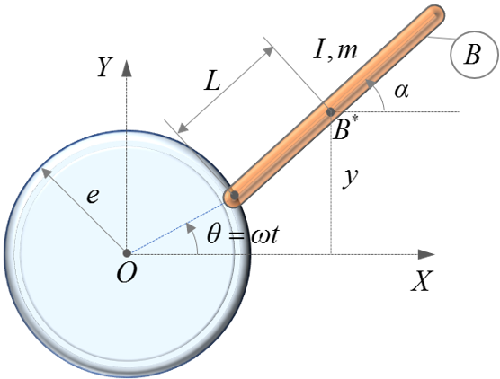
  • Choose the angle of the blade to the global X, α, as the state.
  • Alternatively, you can choose the global y-coordinate of point B*, y, as the state.
Even working with exact math, it is shown below that for two equivalent nonlinear representations of the same physical system, the eigenvalues at any operating point are not the same.
State α State y
Equations of Motion

( I + m L 2 ) α ¨ + m e L ω 2 sin ( α ω t ) = 0 MathType@MTEF@5@5@+= feaagKart1ev2aqatCvAUfeBSjuyZL2yd9gzLbvyNv2CaerbuLwBLn hiov2DGi1BTfMBaeXatLxBI9gBaerbd9wDYLwzYbItLDharqqtubsr 4rNCHbGeaGqipu0Je9sqqrpepC0xbbL8F4rqqrFfpeea0xe9Lq=Jc9 vqaqpepm0xbba9pwe9Q8fs0=yqaqpepae9pg0FirpepeKkFr0xfr=x fr=xb9adbaqaaeGabiGaaiaabeqaamaabaabaaGcbaWaaeWaaeaaca WGjbGaey4kaSIaamyBaiaadYeadaahaaWcbeqaaiaaikdaaaaakiaa wIcacaGLPaaaceaHXoGbamaacqGHRaWkcaWGTbGaamyzaiaadYeaca aHjpWaaWbaaSqabeaacaaIYaaaaOGaci4CaiaacMgacaGGUbWaaeWa aeaacaaHXoGaeyOeI0IaaqyYdiaadshaaiaawIcacaGLPaaacqGH9a qpcaaIWaaaaa@4D70@

 
Operation Point

t = 0 ,   α =0,  α ˙ = ω MathType@MTEF@5@5@+= feaagKart1ev2aqatCvAUfeBSjuyZL2yd9gzLbvyNv2CaerbuLwBLn hiov2DGi1BTfMBaeXatLxBI9gBaerbd9wDYLwzYbItLDharqqtubsr 4rNCHbGeaGqipu0Je9sqqrpepC0xbbL8F4rqqrFfpeea0xe9Lq=Jc9 vqaqpepm0xbba9pwe9Q8fs0=yqaqpepae9pg0FirpepeKkFr0xfr=x fr=xb9adbaqaaeGabiGaaiaabeqaamaabaabaaGcbaGaamiDaiabg2 da9iaaicdacaGGSaGaaeiiaiaaeg7acaqG9aGaaeimaiaabYcacaqG GaGabqySdyaacaGaeyypa0JaaqyYdaaa@417C@

Operation Point

t = 0 ,   y = 0 ,   y ˙ = ( e + L ) ω MathType@MTEF@5@5@+= feaagKart1ev2aqatCvAUfeBSjuyZL2yd9gzLbvyNv2CaerbuLwBLn hiov2DGi1BTfMBaeXatLxBI9gBaerbd9wDYLwzYbItLDharqqtubsr 4rNCHbGeaGqipu0Je9sqqrpepC0xbbL8F4rqqrFfpeea0xe9Lq=Jc9 vqaqpepm0xbba9pwe9Q8fs0=yqaqpepae9pg0FirpepeKkFr0xfr=x fr=xb9adbaqaaeGabiGaaiaabeqaamaabaabaaGcbaGaamiDaiabg2 da9iaaicdacaGGSaGaaeiiaiaadMhacqGH9aqpcaaIWaGaaiilaiaa bccaceWG5bGbaiaacqGH9aqpdaqadaqaaiaadwgacqGHRaWkcaWGmb aacaGLOaGaayzkaaGaaqyYdaaa@4578@

[A] Matrix

A = [ 0 m e L ω 2 I + m L 2 1 0 ] MathType@MTEF@5@5@+= feaagKart1ev2aqatCvAUfeBSjuyZL2yd9gzLbvyNv2CaerbuLwBLn hiov2DGi1BTfMBaeXatLxBI9gBaerbd9wDYLwzYbItLDharqqtubsr 4rNCHbGeaGqipu0Je9sqqrpepC0xbbL8F4rqqrFfpeea0xe9Lq=Jc9 vqaqpepm0xbba9pwe9Q8fs0=yqaqpepae9pg0FirpepeKkFr0xfr=x fr=xb9adbaqaaeGabiGaaiaabeqaamaabaabaaGcbaGaamyqaiabg2 da9maadmaabaqbaeqabiGaaaqaaiaaicdaaeaacqGHsisldaWcaaqa aiaad2gacaWGLbGaamitaiaaeM8adaahaaWcbeqaaiaaikdaaaaake aacaWGjbGaey4kaSIaamyBaiaadYeadaahaaWcbeqaaiaaikdaaaaa aaGcbaGaaGymaaqaaiaaicdaaaaacaGLBbGaayzxaaaaaa@4628@

[A] Matrix

A = [ 0 m e L ω 2 I + m L 2 ω 2 1 0 ] MathType@MTEF@5@5@+= feaagKart1ev2aqatCvAUfeBSjuyZL2yd9gzLbvyNv2CaerbuLwBLn hiov2DGi1BTfMBaeXatLxBI9gBaerbd9wDYLwzYbItLDharqqtubsr 4rNCHbGeaGqipu0Je9sqqrpepC0xbbL8F4rqqrFfpeea0xe9Lq=Jc9 vqaqpepm0xbba9pwe9Q8fs0=yqaqpepae9pg0FirpepeKkFr0xfr=x fr=xb9adbaqaaeGabiGaaiaabeqaamaabaabaaGcbaGaamyqaiabg2 da9maadmaabaqbaeqabiGaaaqaaiaaicdaaeaacqGHsisldaWcaaqa aiaad2gacaWGLbGaamitaiaaeM8adaahaaWcbeqaaiaaikdaaaaake aacaWGjbGaey4kaSIaamyBaiaadYeadaahaaWcbeqaaiaaikdaaaaa aOGaeyOeI0IaaqyYdmaaCaaaleqabaGaaGOmaaaaaOqaaiaaigdaae aacaaIWaaaaaGaay5waiaaw2faaaaa@495A@

Eigenvalues for: m = 3 ,   e = 2 ,   I = 10 ,   L = 10 ,   ω = 10   MathType@MTEF@5@5@+= feaagKart1ev2aqatCvAUfeBSjuyZL2yd9gzLbvyNv2CaerbuLwBLn hiov2DGi1BTfMBaeXatLxBI9gBaerbd9wDYLwzYbItLDharqqtubsr 4rNCHbGeaGqipu0Je9sqqrpepC0xbbL8F4rqqrFfpeea0xe9Lq=Jc9 vqaqpepm0xbba9pwe9Q8fs0=yqaqpepae9pg0FirpepeKkFr0xfr=x fr=xb9adbaqaaeGabiGaaiaabeqaamaabaabaaGcbaGaamyBaiabg2 da9iaaiodacaGGSaGaaeiiaiaadwgacqGH9aqpcaaIYaGaaiilaiaa bccacaWGjbGaeyypa0JaaGymaiaaicdacaGGSaGaaeiiaiaadYeacq GH9aqpcaaIXaGaaGimaiaacYcacaqGGaGaaqyYdiabg2da9iaaigda caaIWaGaaeiiaaaa@4B88@

λ 1 , 2 = ± i m e L 1 + m L 2   ω = ± 4.3994 i MathType@MTEF@5@5@+= feaagKart1ev2aqatCvAUfeBSjuyZL2yd9gzLbvyNv2CaerbuLwBLn hiov2DGi1BTfMBaeXatLxBI9gBaerbd9wDYLwzYbItLDharqqtubsr 4rNCHbGeaGqipu0Je9sqqrpepC0xbbL8F4rqqrFfpeea0xe9Lq=Jc9 vqaqpepm0xbba9pwe9Q8fs0=yqaqpepae9pg0FirpepeKkFr0xfr=x fr=xb9adbaqaaeGabiGaaiaabeqaamaabaabaaGcbaGaaq4UdmaaBa aaleaacaaIXaGaaiilaiaaikdaaeqaaOGaeyypa0JaeyySaeRaamyA amaakaaabaWaaSaaaeaacaWGTbGaamyzaiaadYeaaeaacaaIXaGaey 4kaSIaamyBaiaadYeadaahaaWcbeqaaiaaikdaaaaaaaqabaGccaqG GaGaaqyYdiabg2da9iabgglaXkaaisdacaGGUaGaaG4maiaaiMdaca aI5aGaaGinaiaadMgaaaa@4EC1@

Eigenvalues for: m = 3 ,   e = 2 ,   I = 10 ,   L = 10 ,   ω = 10   MathType@MTEF@5@5@+= feaagKart1ev2aqatCvAUfeBSjuyZL2yd9gzLbvyNv2CaerbuLwBLn hiov2DGi1BTfMBaeXatLxBI9gBaerbd9wDYLwzYbItLDharqqtubsr 4rNCHbGeaGqipu0Je9sqqrpepC0xbbL8F4rqqrFfpeea0xe9Lq=Jc9 vqaqpepm0xbba9pwe9Q8fs0=yqaqpepae9pg0FirpepeKkFr0xfr=x fr=xb9adbaqaaeGabiGaaiaabeqaamaabaabaaGcbaGaamyBaiabg2 da9iaaiodacaGGSaGaaeiiaiaadwgacqGH9aqpcaaIYaGaaiilaiaa bccacaWGjbGaeyypa0JaaGymaiaaicdacaGGSaGaaeiiaiaadYeacq GH9aqpcaaIXaGaaGimaiaacYcacaqGGaGaaqyYdiabg2da9iaaigda caaIWaGaaeiiaaaa@4B88@

λ 1 , 2 = ± i m e L 1 + m L 2 + 1   ω = ± 10.92496 i MathType@MTEF@5@5@+= feaagKart1ev2aqatCvAUfeBSjuyZL2yd9gzLbvyNv2CaerbuLwBLn hiov2DGi1BTfMBaeXatLxBI9gBaerbd9wDYLwzYbItLDharqqtubsr 4rNCHbGeaGqipu0Je9sqqrpepC0xbbL8F4rqqrFfpeea0xe9Lq=Jc9 vqaqpepm0xbba9pwe9Q8fs0=yqaqpepae9pg0FirpepeKkFr0xfr=x fr=xb9adbaqaaeGabiGaaiaabeqaamaabaabaaGcbaGaaq4UdmaaBa aaleaacaaIXaGaaiilaiaaikdaaeqaaOGaeyypa0JaeyySaeRaamyA amaakaaabaWaaSaaaeaacaWGTbGaamyzaiaadYeaaeaacaaIXaGaey 4kaSIaamyBaiaadYeadaahaaWcbeqaaiaaikdaaaaaaOGaey4kaSIa aGymaaWcbeaakiaabccacaaHjpGaeyypa0JaeyySaeRaaGymaiaaic dacaGGUaGaaGyoaiaaikdacaaI0aGaaGyoaiaaiAdacaWGPbaaaa@51E9@

Let MARKER 34 be placed at B*. Its x-axis is along the blade length, and its z-axis along the global z.

To force MotionSolve to use α as the state for linearization:
  1. Define α in a VARIABLE:
    <Reference_Variable id = "22"  type = "EXPRESSION"  expr = "AZ(34)"            />
  2. Tell MotionSolve to use α to generate the linearized equations:
    <Reference_PlantState id = “3010”  num_element = “1”    variable_id_LIST = “22”/>
The MotionSolve results from an eigenvalue analysis are:
NUMBER   NATURAL_FREQ(HZ)  DAMPING_RATIO     REAL(HZ)          IMAG_FREQ(HZ)
     1   7.001886E-01      0.000000E+00      0.000000E+00      7.001886E-01
     1   7.001886E-01      0.000000E+00      0.000000E+00     -7.001886E-01
Note: 7.001886E-01 HZ = 4.39941472 rad/s
The MotionSolve results from a state matrix analysis are:
A = [0.00000000000000000E+00, 1.00000000000000000E+00;
    -1.93548505949367993E+01,-1.91975649453440089E-06]
To force MotionSolve to use y as the state for linearization:
  1. Define y in a VARIABLE:
    <Reference_Variable id = "22"  type = "EXPRESSION"  expr = "DY(34)"            />
  2. Tell MotionSolve to use y to generate the linearized equations:
    <Reference_PlantState id = “3010”  num_element = “1”    variable_id_LIST = “22”    />
The MotionSolve results from an eigenvalue analysis are:
NUMBER   NATURAL_FREQ(HZ)  DAMPING_RATIO     REAL(HZ)          IMAG_FREQ(HZ)
     1   1.738762E+00      0.000000E+00      0.000000E+00      1.738762E+00
     1   1.738762E+00      0.000000E+00      0.000000E+00     -1.738762E+00
The MotionSolve results from a state matrix analysis are:
A = [0.00000000000000000E+00, 1.00000000000000000E+00;
    -1.19354838709666097E+02, 1.71456230219270937E-13]
Note: 1.738762E+00 HZ = 10.9249639 rad/s