
Control: Plant Input
Model ElementThe Control_PlantInput element defines the inputs to a mechanical system or plant.
Description
This is part of the information necessary to create a linearized model of the plant or for co-simulation. You also need to specify the outputs to the plant using the Control_PlantOutput element. Given the inputs and outputs, you may use the Simulate command of type Linear to compute the matrices in the following linearized, state space form:
x is the state vector, u is the input variable, and y is the output variable. A, B, C, and D denote the state matrix, the input matrix, the output matrix, and the direct feed-through matrix, respectively. These matrices are often useful as a starting point in control systems design.
Format
<Control_PlantInput
   id                          = "integer"
 [ label                       = "string" ]
   num_element                 = "integer"
   variable_id_list            = "integer, integer, ..., integer"
 [ hold_order                  = "integer" ]
 [ sampling_period             = "real" ]
 [ offset_time                 = "real" ]
 {
   usrsub_dll_name             = "string"
   usrsub_fnc_name             = "string"
   usrsub_param_string         = "USER([par_1, ..., par_n])"
 |
   interpreter                 = "string"
   script_name                 = "string"
   usrsub_fnc_name             = "string"
   usrsub_param_string         = "USER([par_1, ..., par_n])"
 }
/>
Attributes
- id
- Element identification number (integer>0). This number is unique among all Control_PlantInput elements.
- label
- The name of the Control_PlantInput element.
- num_element
- Number of inputs to the plant that are to be specified using this Control_PlantInput element. num_element > 0.
- hold_order
- Specifies the order of interpolation applied to the control signal(s) propagating out from Control_PlantInput. The default value is 1.0.
- variable_id_list
- Specifies the list of IDs of the variables that define the inputs to the plant. The length of this list is equal to num_element.
- sampling_period
- Specifies the sample time of an input port. A value of 0.0 specifies continuous sampling while any other non-zero value specifies discrete sampling. This value cannot be negative. The default value is 0.0. In most cases, this value need not be changed from its default, except in models where a discrete sampling is required. This parameter is to be used only in the case of co-simulation with MATLAB/Simulink. 3
- offset_time
- Specifies the sample time offset for each input port. The sample time offset must be strictly less than the sampling_period if the latter is non-zero. If the sampling_period is 0.0 (continuous), then offset_time defaults to 0.0 as well. In most cases, this value need not be changed from its default, except in models where a discrete sampling is required. This parameter is to be used only in case of co-simulation with MATLAB/Simulink.
- usrsub_dll_name
- Specifies the path and name of the DLL or shared library containing the user subroutine. MotionSolve uses this information to load the user subroutine in the DLL at run time. Use this keyword only when type = USERSUB.
- usrsub_fnc_name
- This parameter allows you to specify the name for the user subroutine. The default name, PINSUB, is used when the attribute is not specified. Use this keyword only when type = USERSUB.
- interpreter
- Specifies the interpreted language that the user script is written in (example: "PYTHON"). See User-Written Subroutines for a list of valid interpreted languages.
- script_name
- Specifies the path and name of the user written script that contains the routine specified by usrsub_fnc_name.
- usrsub_param_string
- The list of parameters that are passed from the data file to the user- defined PINSUB. Use this keyword only when type = USERSUB. Set this parameter equal to "USER(parameter 1, par 2,..., par n)", where the parameters are chosen by you.
Example
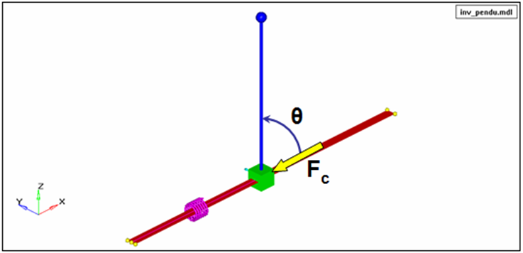
- Plant input: Control force (Fc) acting on slider along global X.
- Plant output: Pendulum angle θ.
The plant input may be defined as follows:
<Control_PlantInput
    id                = "303001"
    num_element       = "1"
    variable_id_list  = "6"
    hold_order        = "1"
/>
Reference_Variable 6 defines the control force (Fc).
<Reference_Variable
   id         = "6"
   type       = "EXPRESSION"
   expr       = "0.0"
/>
Comments
- The output specified using the Control_PlantInput element can be accessed using the function PINVAL. This function can be called directly from within MotionSolve expressions and used from within user subroutines using SYSFNC() and SYSARY().
-
Control_PlantOutput and Control_PlantInput are used for co-simulation. This is a scenario where a problem is split between two solvers. The two solvers work in tandem to solve the problem, exchanging information as required by them with Control_PlantOutput and Control_PlantInput objects. A common scenario is the control of a mechanical system. The control system is modeled in controls software and the mechanical system in MotionSolve. The mechanical system tells the controller what it is doing; the controller uses this to determine the control forces to apply. This information is exchanged continuously or at discrete sampling steps. Control_PlantInput tells MotionSolve what the controller inputs to the model are. Control_PlantOutput tells MotionSolve what information to send to the controller. The user subroutine options are used for co-simulation. For more information on co-simulation, see Couple MotionSolve with Other Software.
- A discrete (only) system in Simulink will require that the sampling_period be set to a discrete time (for example, non-zero; zero is continuous sampling). Otherwise, the simulation will not run and an error will occur.
- For co-simulation from a Simulink-driven model, create the number of Control_PlantInput's in a manner that is convenient to you, and the S-Function that represents the MotionSolve model will update accordingly. See MV-7002: Co-simulation with Simulink for an example.
- For a co-simulation with a Simulink Coder library, create as many Control_PlantInput's as Outports (for example, one Control_PlantInput for each Outport; the output of the Simulink model is the input to the MotionSolve (plant) model) in the Simulink model to setup the proper interface communication. See MV-7005: Linking Matlab/Simulink Generated Code (Simulink Coder) with MotionSolve for an example.
- The order of the Control_PlantInput's found in the MotionSolve model (.xml) (by line number, from top to bottom) should match the order of the IDs for the Outports in the Simulink model to ensure the variables are exchanged in the proper order. The same is true for the order of the inputs to an S-Function for a Simulink-driven co-simulation.
- For a Simulink Coder library co-simulation, set usrsub_param_string to have one integer that will uniquely identify the Simulink Coder library used. This number (ID) should be the same for all Control_PlantInput's and Control_PlantOutput's that are used for this Simulink Coder library.