Force: Penalty
Model ElementForce_Penalty defines a generalized force whose purpose is to maintain a "soft" constraint in the system.
Description
This means that when the constraint is satisfied, there is no penalty force. However, if the constraint is violated, a penalty force that tries to reduce the violation is generated. The generalized force acts on all the coordinates involved in the definition of the constraint.
Format
<Force_Penalty
       id                  = "integer"
      [label               = "string"]
       penalty             = "double"
      [penalty1            = "double"]

     [[
       unilateral          = "False" | "True"
       smoothing_factor    = "real"
     ]]

     {
       type                = "EXPRESSION"
       expr                = "motionsolve_expression"

       type                = "USERSUB"
       usrsub_dll_name     = "valid_path_name"
       usrsub_fnc_name     = "custom_fnc_name"
       usrsub_param_string = "USER(par_1, ..., par_n)"

       type                = "USERSUB"
       script_name         = "valid_path_name"
       interpreter         = "string"
       usrsub_fnc_name     = "custom_fnc_name"
       usrsub_param_string = "USER(par_1, ..., par_n)"
     }
/>
Attributes
- id
- Specifies the element identification number (integer>0). This number is unique among all Reference_Variable elements.
- label
- This attribute describes the name of the Reference_Variable element. The description is primarily used to make the input more readable.
- penalty
- Specifies a penalty factor to be used in calculating the restoring force that is used to enforce that the algebraic constraint is always zero. penalty > 0. 2
- penalty1
- Specifies a second penalty factor to be used in calculating the restoring force that is used to enforce that the time derivative of the algebraic constraint. The default value for penalty1 is zero. When specified, penalty1 ≥ 0. 3
- unilateral
- A Boolean attribute. Select one from TRUE and FALSE. Indicates whether an equality constraint, or an inequality constraint is being specified. unilateral is an optional attribute. If defaults to FALSE when not specified. 1 4
- smoothing_factor
- The penalty force due to a unilateral constraint is ramped up in a smooth manner using a STEP function. This specifies the x-value at which the smoothing is completed. smoothing_factor > 0. 4
- type
- Select from EXPRESSION and USERSUB. Specifies how the
constraint governing the penalty force is defined.
- EXPRESSION
- Specifies that the constraint is defined in a MotionSolve expression that can be evaluated at run-time.
- USERSUB
- Indicates that the algebraic constraint is specified in a user-defined subroutine.
- expr
- Specifies the MotionSolve expression that defines the algebraic constraint. Use this attribute only when type= EXPRESSION. Any valid run-time MotionSolve expression can be provided as input.
- usrsub_dll_name
- Specifies the path and name of the DLL or shared library containing the user subroutine. MotionSolve uses this information to load the user subroutine in the DLL at run time. Use this keyword only when type = USERSUB.
- usrsub_fnc_name
- This parameter allows you to specify the name for the user subroutine. The default name, PFOSUB, is used when the attribute is not specified. Use this keyword only when type = USERSUB.
- usrsub_param_string
- The list of parameters that are passed from the data file to the user-defined PFOSUB. Use this keyword only when type = USERSUB.
- script_name
- Specifies the path and name of the user written script that contains the function specified by usrsub_fnc_name. Use this keyword only when type = USERSUB.
- interpreter
- Specifies the interpreted language that the user script is written in (example: "PYTHON"). See User-Written Subroutines for a choice of valid interpreted languages. Use this attribute only when type = USERSUB.
Example 1
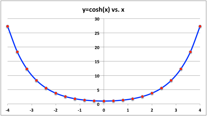
Assume a bead, modeled as a particle, is sliding on a catenary fixed in the global x-y plane as shown in Figure 1. The path of the bead is shown as a red circle, and the catenary as a blue line.

The constraint is represented as: g(x,y) = y - cosh(x) = 0.
The time derivative of the constraint is: g(ẋ,ẏ,x,y) = ẏ - sinh(x)ẋ = 0.
Let MARKER 9 represent the center of mass of the bead. Assume a penalty of 1E4 is used to enforce the constraint, and a penalty of 1E2 to enforce the time derivative of the constraint. The MotionSolve Force_Penalty statement is:
<Force_Penalty
     id       = "1"
     label    = "Particle sliding on a catenary"
     type     = "EXPRESSION"
     expr     = "dy(9) - cosh(dx(9))"
     penalty  = "1E4"
     penalty1 ="1E2"
/>
The displacement constraint for the penalty force is:
g = dy(9)-cosh(dx(9))The velocity constraint for the penalty force is:
ġ= vy(9)-sinh(dx(9)*vx(9)The penalty force that is computed by MotionSolve is:
F = -1E4*g - 1E2*ġ
  = -1E4*[dy(9)-cosh(dx(9)] -1E2*[vy(9)-sinh(dx(9))*vx(9)]
Example 2
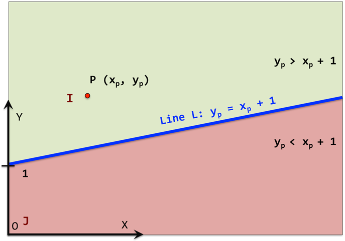
This example demonstrates how a simple unilateral constraint can be implemented with Force_Penalty. Figure 2 below shows a line L, y=1+x, defined in the coordinate system of a Marker, J.

J has origin O, x-axis along X and y-axis along Y. A point P, belonging to another body, has coordinates (xp,yp) as measured in J. For the sake of convenience, define a Marker I=10, whose origin is at P.
- Define the inequality constraint that captures this requirement.
- Define a Force_Penalty to apply a contact force dependent on the
penetration and penetration velocity.
From simple coordinate geometry considerations, we can see that:
- The green region, of permissible motion, is is represented by: yp > 1 + xp
- The red region, of impermissible motion, is represented by: yp < 1 + xp
- The boundary between these regions is represented by line L: yp = 1 + xp
The constraint we wish to impose is: yp ≥ 1 + xp or 1 + xp - yp ≤ 0
The Force_Penalty definition is therefore:
<Force_Penalty
    id                 = "10"
    label              = "Enforce 1+x < = y"
    type               = "EXPRESSION"
    expr               = "1 + dx(10) - dy(10)"
    penalty            = "1E4"
    penalty            = "1E2"
    unilateral         = "True"
    smoothing_factor   = "1.0"
/>
Example 3
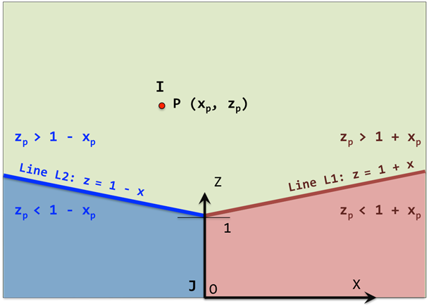
This example demonstrates how a simple unilateral constraint can be implemented with Force_Penalty. Figure 3 shows a line L, y=1+x, defined in the coordinate system of a Marker, J.

- Define the inequality constraints that captures this requirement.
- Define two Force_Penalty to enforce these constraints.
- The green region, of permissible motion above L1, is represented by: zp > 1 + xp
- The red region, of impermissible motion below L1, is represented by: zp < 1 + xp
- The boundary between these regions is represented by line L1: zp = 1 + xp
- The green region, of permissible motion above L2, is represented by: zp > 1 - xp
- The blue region, of impermissible motion below L2, is represented by: zp < 1 - xp
- The boundary between these regions is represented by line L2: zp = 1 - xp
- zp ≥ 1 + xpor1 + xp - zp ≤ 0
- zp ≥ 1 - xpor1 - xp - zp ≤ 0
The Force_Penalty definitions are therefore:
<Force_Penalty                            |<Force_Penalty
   id               = "1"                 |      id               = "2"
   label            = "Enforce 1+x<=z"    |      label            = "Enforce 1-x<=z"
   type             = "EXPRESSION"        |      type             = "EXPRESSION"
   expr             = "1+dx(10)-dz(10)"   |      expr             = "1-dx(10)-dz(10)"
   penalty          = "1E4"               |      penalty          = "1E4"
   penalty1         = "1E2"               |      penalty1         = "1E2"
   unilateral       = "True"              |      unilateral       = "True"
   smoothing_factor = "1.0"               |      smoothing_factor = "1.0"
/>                                        |/>
Figure 4 below shows the X and Z coordinates of particle P (Marker 10), when it starts from an initial condition of Xp=100 mm and Zp=120 mm and falls under the influence of gravity. The acceleration due to gravity is -9810 mm/s2 in the Z direction.
The particle bounces between the two lines and eventually comes to rest at Zp=1 and Xp=0.

Comments
- Force_Penalty may be used to define
unilateral or inequality constraints. Let q be any set
of values dependent on system displacements.
- Equality or bilateral constraints have the form g(q,t) = 0
- Inequality or unilateral constraints have the form g(q,t) ≤ 0
- In both cases, a penalty force is generated only when the constraint is violated.
- For equality constraints when g(q,t) ≠ 0
- For unilateral constraints when g(q,t) > 0
- Assume that a constraint
g(q,t)=0 is to be maintained in the model.
One approach to solve the problem is to define a user-defined constraint and to provide the constraint g(q,t)=0 to MotionSolve. The constraint is enforced by an unknown Lagrange multiplier λ that is solved with the rest of the system variables.
- λ may be a force or a torque.
- λ acts along the gradient of the constraint,
 .
. - The generalized force acting on the system is
 .
. For more information on the above-mentioned approach, see Constraint_General.
Force_Penalty uses a slightly different method to accomplish the same. The constraint is "soft", in other words, it is not strictly enforced. Violations of the constraint are allowed, but a restoring force tending to decrease the constraint violation is internally generated.
- The penalty force may be a force or a torque.
- The penalty force has the magnitude, F = -penalty*g(q,t).
- The penalty force acts along the gradient of the constraint,
 .
. - The generalized force acting on the system is
 .
. - Generally speaking, a large penalty ensures a small constraint
violation.
There is a close correspondence between a hard constraint with a Lagrange Multiplier and a soft constraint with a penalty force.
- If g(q,t)=0, then it
automatically implies ġ(q̇,,q,t)=0, where
ġ(...) =
 . q̇ are
the velocities corresponding to q.To enforce ġ(q̇,,q,t)=0, a second component -penalty1*ġ(q̇,,q,t) must be added to the penalty force computed earlier. To enforce both g(q,t)=0 and ġ(q̇,,q,t)=0, the following strategy is used:
. q̇ are
the velocities corresponding to q.To enforce ġ(q̇,,q,t)=0, a second component -penalty1*ġ(q̇,,q,t) must be added to the penalty force computed earlier. To enforce both g(q,t)=0 and ġ(q̇,,q,t)=0, the following strategy is used:- The penalty force has the magnitude, F = -penalty*g(q,t) - penalty1*ġ(q̇,,q,t).
- The penalty force acts along the gradient of the constraint,
 .
. - The generalized force acting on the system is
 .
. When penalty1 is specified, MotionSolve uses the above equations to compute the penalty force and the generalized forces on the equations of motion.
- A smoothing function is used to smooth the equations in
3 as follows:
- p = penalty * STEP(g(q),0,0,smoothing_factor,1)
- p1 = penalty * STEP(g(q),0,0,smoothing_factor,1)
- F = - p*g(q,t) - p1*ġ(q̇,,q,t) )
- The STEP function is used to gradually ramp up the penalty factors as the violations increase. This is shown in Figure 5. The transition will become steeper as smoothing factor becomes smaller.
Figure 5. The Smoothing Factor for Unilateral Constraints
- Three approaches are available for defining the
function g(y,t).
- As a function expression in the XML file: This is probably the simplest approach, and g(y,t) is defined as an expression composed from the built-in functions and operators in the function expression language
- As compiled user-written subroutine, provided in a DLL. Any language may be used. MotionSolve provides an interface to Fortran, C and C++. The default name for the user-written subroutine is PFOSUB. However, you are allowed to give the function any name and tell MotionSolve what it is.
- As a script written in the Python or MATLAB language: Though this approach is slightly less efficient than writing the user-written subroutine in a compiled language, it provides two significant benefits: (A) It provides for a vastly more flexible and powerful environment to compose the function g(y,t) than function expressions, and, (B) There is no need for compilers and linkers as is the case when Fortran, C or C++ are used.
- Excessively large values for penalty and penalty1 can cause numerical difficulties. Think of penalty as being similar to a stiffness and penalty1 to damping.
- Very small values of smoothing_factor may also cause numerical difficulties. A good rule of thumb is to make the smoothing factor a fraction of the maximum penetration expected.
- Constraints of the form h(q,t) ≥
0 may be implemented as follows:
- Define g(q,t) = -h(q,t)
- Impose the penalty constraint on g(q,t) ≤ 0
