Since version 2026, Flux 3D and Flux PEEC are no longer available.
Please use SimLab to create a new 3D project or to import an existing Flux 3D project.
Please use SimLab to create a new PEEC project (not possible to import an existing Flux PEEC project).
/!\ Documentation updates are in progress – some mentions of 3D may still appear.
3D curves dedicated to rotating machines
General information
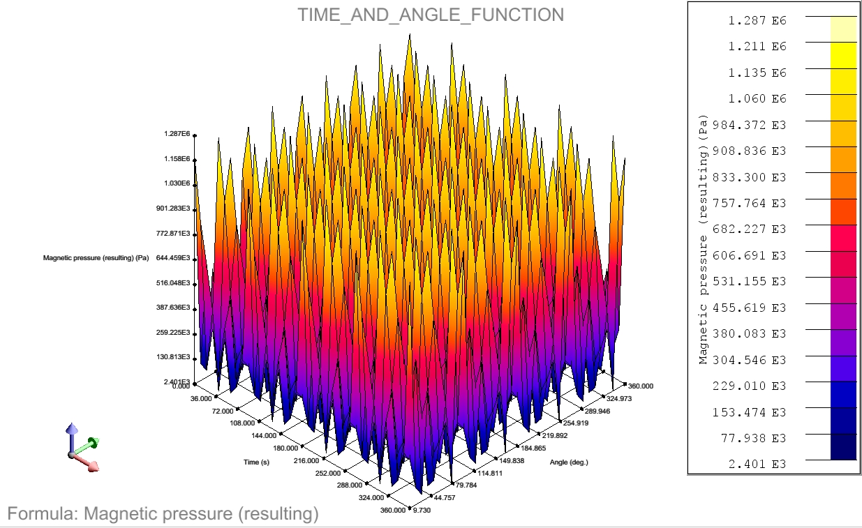
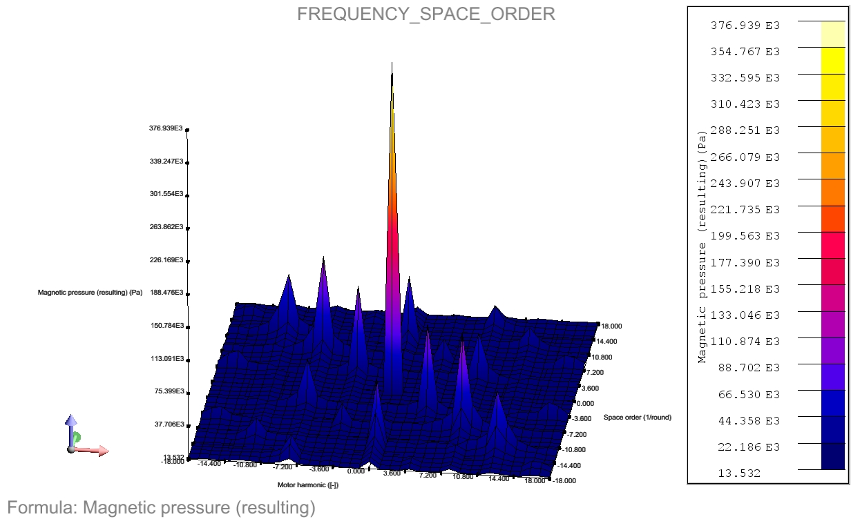
The 3D curves dedicated to rotating machines allow computing a quantity's values along a circle positioned around the rotation axis of a rotating machine, typically in the airgap zone. These values are collected for a set of time steps (feature available only in Transient Magnetic application). Once collected, the values are represented as a 3D plot having in abscissa the time and the angular position along the computation circle. A specific option allows also to transform the time-domain values into a 2D-Fourier domain representation, where data are expressed as a function of the motor-harmonic and the spatial order.Dialog box options
The dialog box for the creation of a 3D curve dedicated to rotating machines is presented below:
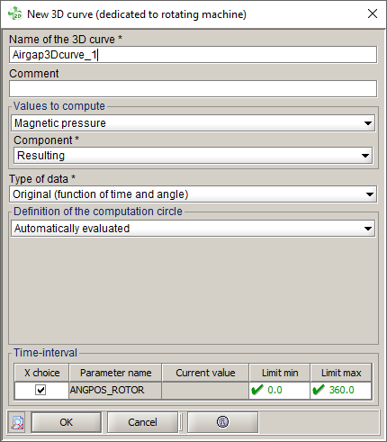
The fields the user has to fill in are as follows:
- Values to compute: the user can choose between:
the Magnetic pressure, which is the most common quantity used in these analysis and which allows to compute the magnetic pressure module or one of its components: radial (also called normal) or tangential.
This magnetic pressure at the computation points is obtained by the following formula:

where the first and second terms represent, respectively, the normal and tangential component of the magnetic pressure.
- and his own User formula, which allows to compute the values of a user defined spatial formula. The quantity expressed by the chosen formula must be real scalar.
- Type of data: the user can choose between:
- Original (function of time and angle), which returns the values in the time/angular position domain.
- Double FFT (function of motor harmonic and space order), which returns the values in the frequency/spatial order domain. Those values are obtained by applying a 2D Fourier transform. The frequencies are normalized by the rotation speed to be expressed in terms of motor-hamonics.
- Definition of the computation circle: in 2D and in Skew, by
default, the computation circle is automatically evaluated by Flux, but the
user can define by himself the parameters by selecting the user defined
option, which indeed is the only one available in 3D. In that user defined
case, illustrated in the picture below, the user is invited to define:
- the Radius of the circle where to compute the selected quantity;
- in case of Skew and 3D applications, the Z position of the computation circle in the airgap;
- the Length unit used for the radius and for the Z position of the computation circle in the airgap;
- the Number of computation points along perimeter, whose default value is set to 1080, which means three points per degree in case of a full rotation.
- Time interval
- Interval, allows to select a set of time (or position) steps. If the data type Double FFT is selected, the interval must represent one complete rotor revolution around its axis to ensure the periodicity of the time evolution.

3D curve examples