Tutorial 8: PID Controller Tutorial

Purpose/Objective

This exercise will walk the user through adding a PID Controller to an already existing model. The user will learn how to:

• Edit PID Controller element properties
• Check the model
• Run the model
• Post-process the model
• Elements used: PID Controller Element

Step 1: Examine geometry and create plan

1. The goal of this exercise is to determine what size the tip cap holes need to be in order to allow a specified flow to pass through. This will be done by adding PID controller elements to the two flow elements representing the tip cap holes. The PID elements will be set to iterate on the area of the conventional orifice elements in order to reach the desired flow rate.
   1. The flow rates of the tip cap holes from the turbine blade model we created earlier, can be seen in Figure 1.02
   2. The goal of this exercise is to use PID Controller elements to distribute the flow rate evenly, so that each hole has a flow rate of 0.014 lb/s

      

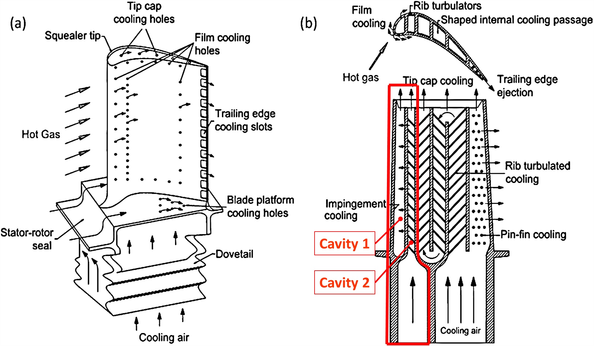
   Figure 1.01: Turbine Blade Cooling Layout

   

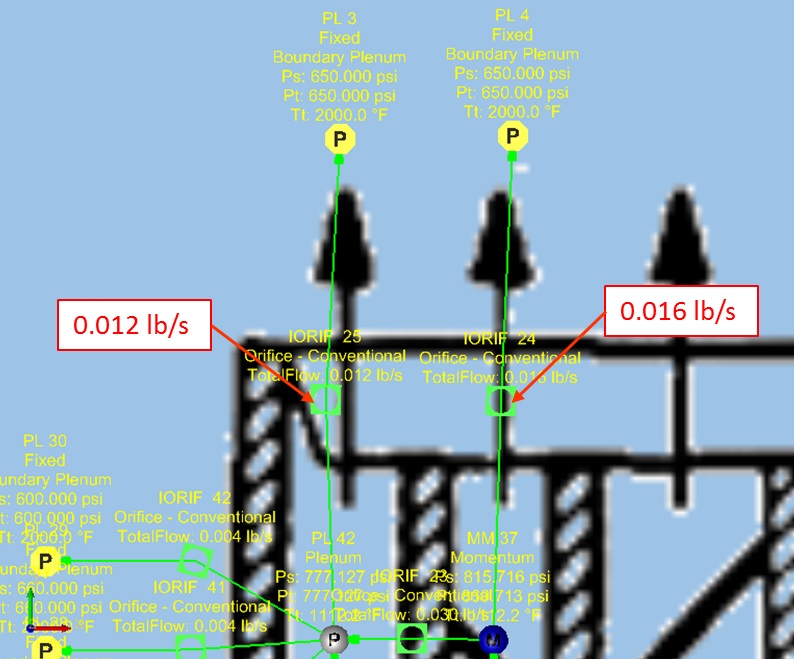
   Figure 1.02: Tip cap hole flow rate from previous example

Step 2: Building Model

1. Start by opening the previously created blade model (Model_Exercise_7_start.flo)

   

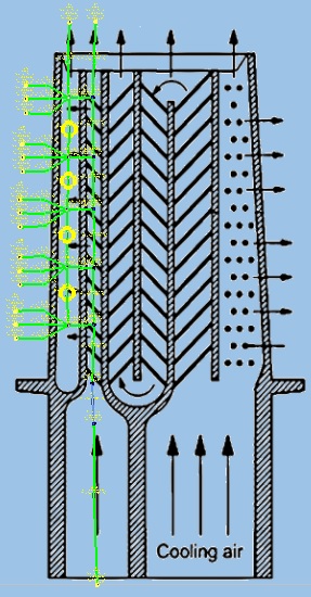
   Figure 1.03: Rotating Cooled Turbine Blade

2. Place a PID Controller Element next to each of the two conventional orifice elements representing the tip cap cooling holes

   

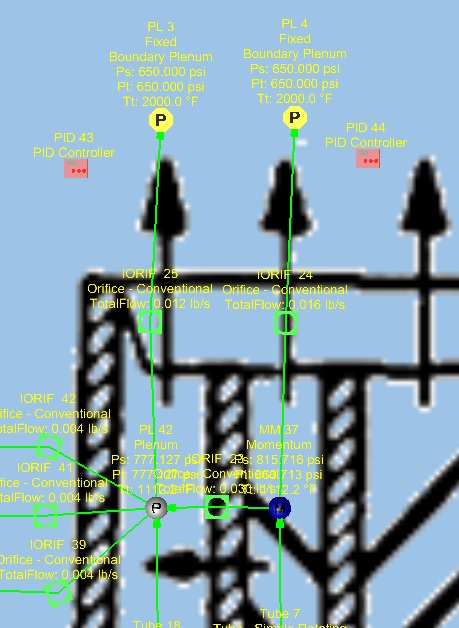
   Figure 1.04: PID Controller element placement

3. For the left PID controller
   1. Set Gauge Variable → Item Type to Element
   2. Set Gauge Variable → Item ID to the element ID of which measurements will be taken from (in this case: 25)
   3. Set Gauge Variable → Property to Mass Flow Total (pps)
   4. Set Gauge Variable → Set Point Variable to 0.014 (this is the flow rate that the controller will try to achieve)
   5. Set Manipulated Variable → Item Type to Element
   6. Set Manipulated Variable → Item ID to the element ID of the element that will be changed in order to achieve the goal flow rate (in this case: 25)
   7. Set Manipulated Variable → Property to Area (in^2)
   8. Set PID Equation Form → Integral Gain Constant to 0.001
   9. Set PID Equation Form → Reset Value(Bias) to 0.2
   10. Set PID Equation Form → Convergence Tolerance to 0.0001
   11. Set Show Advanced Options → Minimum Manipulated Value to 0.001
   12. Set Show Advanced Options → Maximum Manipulated Value to 0.003

   

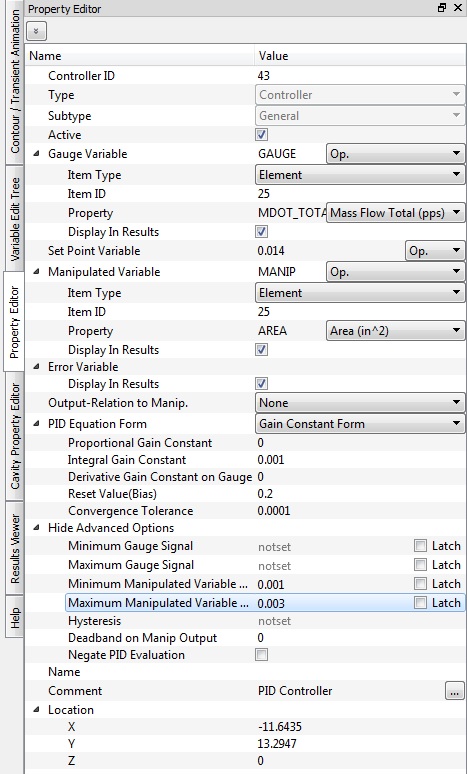
   Figure 1.05: PID Controller element inputs (left)

4. Do the same steps for the right PID controller element

   

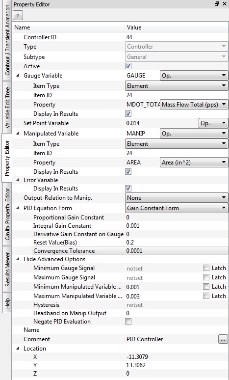
   Figure 1.06: PID Controller element inputs (right)

5. Set Solver → Analysis Setup → Solver Convergence → Maximum Number of Iterations to 1000

Step 3: Check Model and Run

1. Select checkmark icon from the top toolbar to check the model for warnings/errors.
   • An error should populate stating that the internal chamber has not been initialized
2. Select the initialization icon from the toolbar, and pick Start. Accept values once flow solver has converged.
3. Select run icon from toolbar. Run Flow Simulator.

Step 4: Post-process

1. Results file (*.res) should automatically be loaded into GUI. If not, it can be selected via File → Load Result File
2. By default, both chamber and elemental results are displayed in the graphical workspace.

   

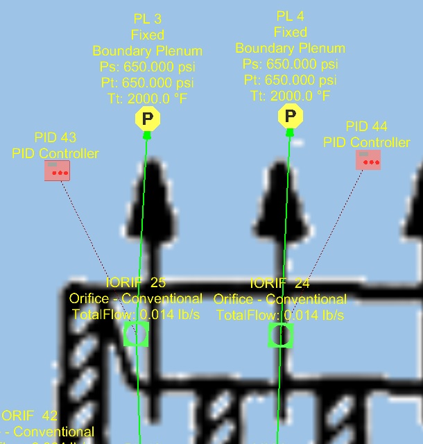
   Figure 1.07: Results showing the target flow rate of 0.014 lb/s has been achieved

3. Open the .res file in the run directory and scroll to the bottom for information on the PID controller elements and to find out the area that was assigned to the orifice elements in order to achieve the target flow

   

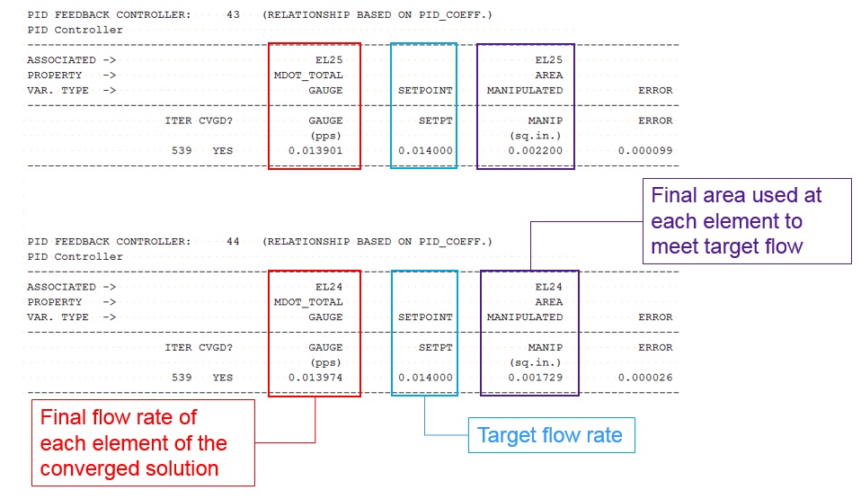
   Figure 1.08: Results showing the area used to achieve the target flow rate at the bottom of the .res file