Tutorial 16: Transient Thermal Network for a 2D metal structure
Purpose/Objective
This exercise will walk the user through building a standalone thermal network for arbitrary 2D metal structure. The user will demonstrate the capability of the thermal network features of Flow Simulator to compare with an analogous MSC Patran-Thermal resistor network and will learn how to:
- Edit thermal chamber properties
- Edit thermal element properties
- Check the model
- Run the model
- Post-process the model
- Thermal Network: Conduction
Step 1: Examine geometry and create plan
- The user will be replicating a thermal model of Thermal nodes (MSC Patran) to
construct an analogous representation of the metal structure. These metal nodes will
then be connected to one another via Conductors to mimic the “metal” resistors
created by MSC Patran-Thermal. The mass of structure included in the model is then
lumped onto each Temperature Node (metal) in a fashion analogous to MSC
Patran-Thermal as well shown in Figure 1.01.
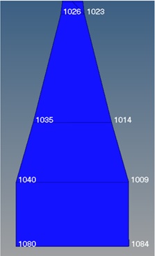
Figure 1.01: 2D Metal surfaced examined in MSC Patran-Thermal
- Patran-Thermal represents a 2D-axysimmetric “quad” element via 4 edge resistors and 2 cross resistors, as shown replicated here in Flow Simulator.
Step 2: Building Model
- Plan model setup based on what is known about the geometry
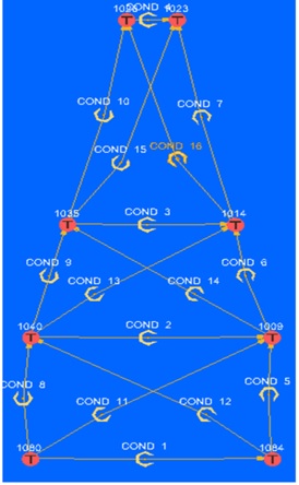
Figure 2.01: Sketch/Outline of building thermal model
- Define metal material from Material Manager

- Select “New Solid”
- Name it as “Custom_Material_1”
- Select Arbitrary Mixture (CoolProp) as Material Type and set Density and Thermal Emissivity
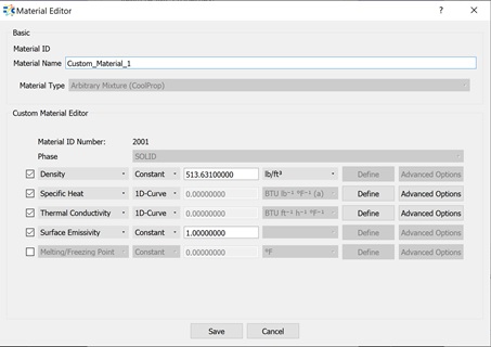
Figure 2.02: User Defined solid material
- Drag and Drop Internal Thermal Nodes at the corners of the 2D metal.
- Renumber
 the thermal nodes to
make the comparison easier.
the thermal nodes to
make the comparison easier. - Set Node Temperature
- Set Volume
- Select Material as “Custom_Material_1”
for all internal T-Nodes
- Renumber
- Connect all the internal tnodes to each other with
 Conductor elements.
- Select Material
- Set Cross-Section Area
- Set thickness
For all Conductors
- Connect Internal Tnodes and Boundary Tnodes with
 Convector element to represent convection
into the system
Convector element to represent convection
into the system- Set Heat Transfer Coefficient
- Set Surface area
- To finish up the model drag and drop 5 Mission BC Controller and connect them to
Boundary Tnodes
- Relation type Table 1D
- GAUGE will be Mission with Property of Time
- MANIPULATED will be the boundary Tnodes with Property of Total
Temperature
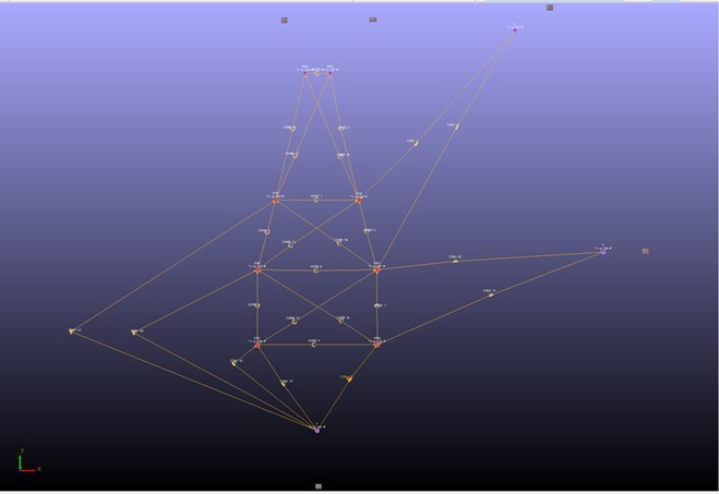
Figure 1.04: Thermal circuit set-up
Step 4: Check Model and Run
- Select checkmark icon from the top toolbar
 to check the model for warnings/errors.
- Error should mention the Analysis Type = Steady State Flow
- Select the initialization icon from the toolbar
 , and pick Start. Accept values once flow
solver has converged.
, and pick Start. Accept values once flow
solver has converged. - For Steady State Comparison: Analysis Setup → Analysis Type = Steady State Thermal
- For Transient comparison: Analysis Setup → Analysis Type = Thermal Transient
- Select run icon from toolbar
 . Run Flow Simulator.
Step 5: Post-process
- Results file (*.res) should automatically be loaded into GUI. If not, it can be selected via File → Load Result File
- Node temperature display may have to be enabled in Settings → Display Options → Thermal Results → Nodal Temperature
- From Post-Processing → Contour/Transient Animation, it is possible to see the results with coloring option
- Figure 1.07 Temperature results benchmarking. The figure on the Right Side shows the temperature of TNodes on Flow Simulator analysis
- Moreover, transient analysis can be plotted from Post-Processing → Results Table →
Create Plot

Figure 5.01: Contour Plot of Thermal results after running model with Flow Simulator
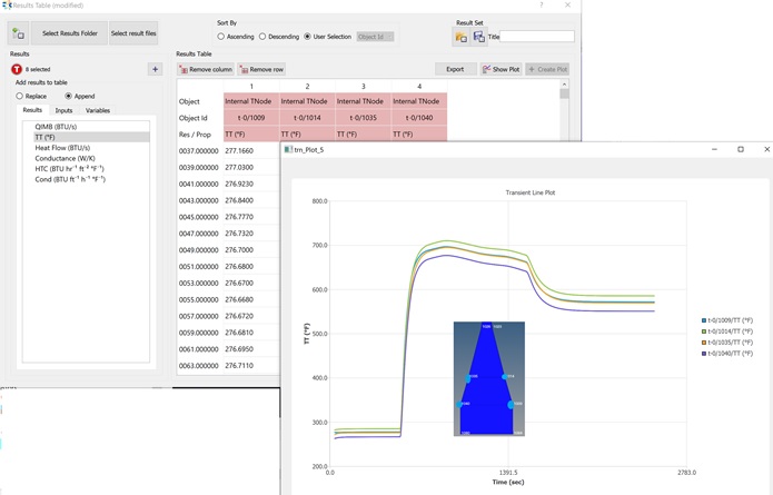
Figure 5.02: Transient analysis plots of nodes at specified points