Tutorial 18: Variable Definition Tutorial
Purpose/Objective
This exercise will walk the user through building a simple tube & orifice model with the use of variable definition. The user will learn how to:
- Create Chamber & Element
- Create Variable & Set Expression
- Define Element Properties via Variable
- Check the model
- Run the model & Post-Process
- Creation of Multi-Case
- Creation of Derived Result Variable
- Post-process of Multi-Case run
- Chamber Types: Plenum, Momentum
- Element Types: Conventional Orifice, Tube
- Fluid: Air
Step 1: Create Chamber & Element
- The user will be creating a flow model consists of simple tube and orifice element where tube radius is known.
- Plan model setup based on what is known about the geometry
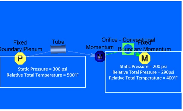
Figure 1.01: Sketch/Outline of model
- Drag and drop Boundary Plenum & Boundary Momentum chambers at the inlet and
outlet locations as shown Figure 1.01
- Translate (right click chamber/element → translate) option and manually editing the coordinates (Property Editor → Location), can be used to assist in placing chambers and elements in the right location
- Use
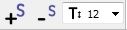 to adjust symbol and text size
 - Place non-boundary momentum chambers at the center location.
- Connect stationary tube element between boundary plenum (left) and the center momentum chamber, and conventional orifice element between center momentum chamber and boundary momentum (right) chamber.
- For the inlet boundary plenum
- Set pressure to 300 psi
- Set temperature to 500 F
- For the sink boundary momentum
- Set static pressure to 200 psi
- Set total pressure to 290 psi
- Set temperature to 400 F
- For the outlet conventional orifice
- Set area to 0.25 in^2
- Set Cd to 0.8
Step 2: Create Variable and Expressions
- Creation of Variable
- Click
 to open Variable
Edit Tree or the steps described in quick guide
to open Variable
Edit Tree or the steps described in quick guide - Create Variable named “Radius” and set a constant value of 0.25
- Create another variable named “Area” and set expression as
“Math.pow([Radius],2) *Math.PI” in secondary pop-up window as shown in
the following figure. Make sure to click “Execute” button after
defining.
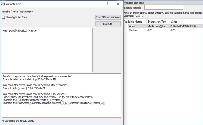 Figure
1.02
Figure
1.02
- Click
Step 3: Define Element properties via Variable
- For the Tube Element
- Set Geometric Input Type as “Area” only
- Set Geometric Input size as “Constant” only
- Set Area as “[Area]”, which is a defined variable, as shown Figure 1.03
- Set Length as 5 in.
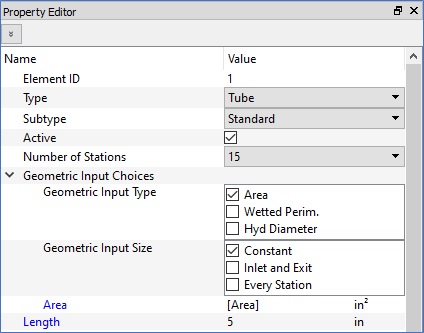
Figure 1.03
Step 4: Check Model and Run
- Select checkmark icon from the top toolbar
 to check the model for warnings/errors.
- An error should populate stating that the internal chamber has not been initialized
- Select the initialization icon from the toolbar
 , and pick Start. Accept values once flow
solver has converged.
, and pick Start. Accept values once flow
solver has converged. - Select run icon from toolbar
 . Run Flow Simulator.
Step 5: Post-process
- Results file (*.res) should automatically be loaded into GUI. If not, it can be selected via File → Load Result File
- By default, both chamber and elemental results are displayed in the graphical
workspace.
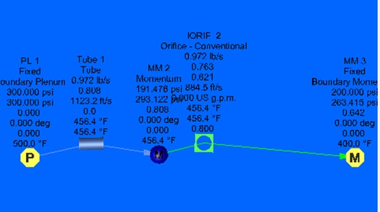
Figure 1.04: Model results
- Results displayed after running the model will include pressures, temperatures, and swirl values
Step 6: Creation of Multi-Case & Run
- In this section a multicase will be created using MultiCase Creator Tool with 4 case where in each case Cd values of the orifice element will be varied (0.2, 0.4, 0.6 & 0.8).
- Click
 to open Multicase Creator Graphical User
Interface.
to open Multicase Creator Graphical User
Interface. - Click “Properties” tab on left side of the GUI Window.
- Select Orifice element from main Graphic window, when selected the properties related to the element will be populated in left side of the Multicase Creator GUI
- Select “Discharge Coefficient(CD) (HeadLoss)” from the list of items.
- Click
 4 times to add 4 columns in left
side of the table.
4 times to add 4 columns in left
side of the table. - Enter 0.2, 0.4, 0.6 & 0.8 for Case 1 , Case 2, Case 3 & Case 4 column.
- Save the multi-case by clicking
 in top left corner of the Multicase Creator
GUI.
in top left corner of the Multicase Creator
GUI.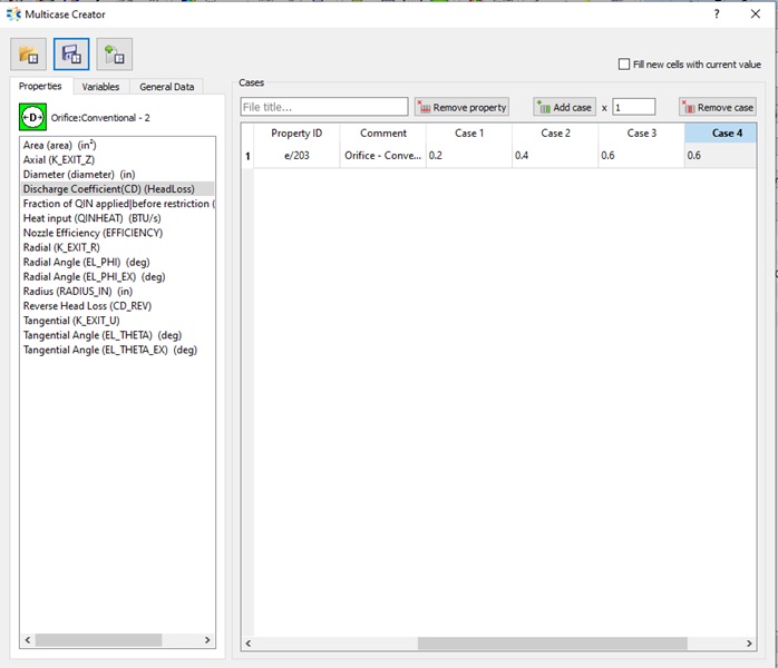
Figure 1.05: Multi-Case Creator
- Select the initialization icon from the toolbar, and pick Start. Accept values once flow
solver has converged.
- Select run icon from toolbar.
- Choose “Multiple Cases” and click “Multi-Case Settings” button to make sure proper multicase import file is selected.
- Check “Save Results to separate Folder” and then Run Flow Simulator
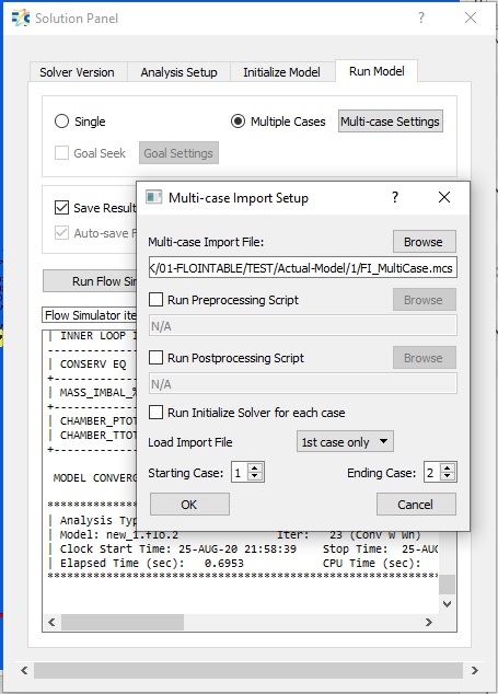
Figure 1.06: Run option during Multi-Case
Step 7: Creation of Derived Result Variable
- In this section a result variable will be created using Variable Edit Tool
- Open Variable Edit Tree by clicking
 button.
 - Create a new variable named “Dynamic-Head”. Right-Click and then “Set Expression” to
define the expression for this newly created variable.
- Click “Insert Result Variable” button.
- Select “Chamber”.
- Select “Entity” from drop-down list.
- “Select “Total Pressure” from the populated list.
- Click “Insert Expression”.
- Enter “-” (negative sign) inside the expression box.
- Repeat process (i-v) to insert static pressure. After the expression should looks like as shown in figure 1.07.
- Click Execute.
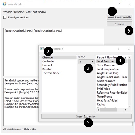
Figure 1.07: Defining Derived result variable
Step 8: Post-Process Multi-case Result using Result Table
- This section will provide details on how to post-process multi-case results with one
derived result variable
- Open “Result Table” pop-up GUI by clicking
 button.
 - Click “Select Result Folder” to choose the multi-case result folder.
- Click “Variable” Tab under which all defined variables are listed.
- Choose “Dynamics-Head”. The “Dynamic-Head” data of all 4 cases will be displayed in right window as shown in the figure 1.08.
- User can create plot using
 option
 - At last user can save the result set by clicking
 button.
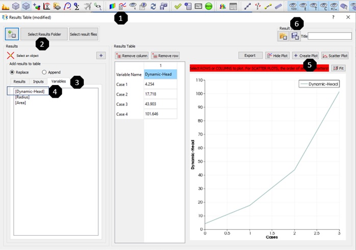
Figure 1.08: Defining Derived result variable
- Open “Result Table” pop-up GUI by clicking