Tutorial 4: Cooling circuit of a rotating turbine blade
Purpose/Objective
This exercise will walk the user through building a portion of the cooling circuit of a turbine blade, based on the defined geometry. The user will learn how to:
- Edit chamber properties
- Edit element properties
- Check the model
- Run the model
- Post-process the model
- Chamber Types: Plenum and Momentum
- Element Types: Simple Rotating Tube, Conventional Orifice
- Fluid: Air
Step 1: Examine geometry and create plan
- We will be creating a model of the cooling circuit of the Leading Edge (LE) of a High-Pressure Turbine Blade (highlighted red in figure 1.01).
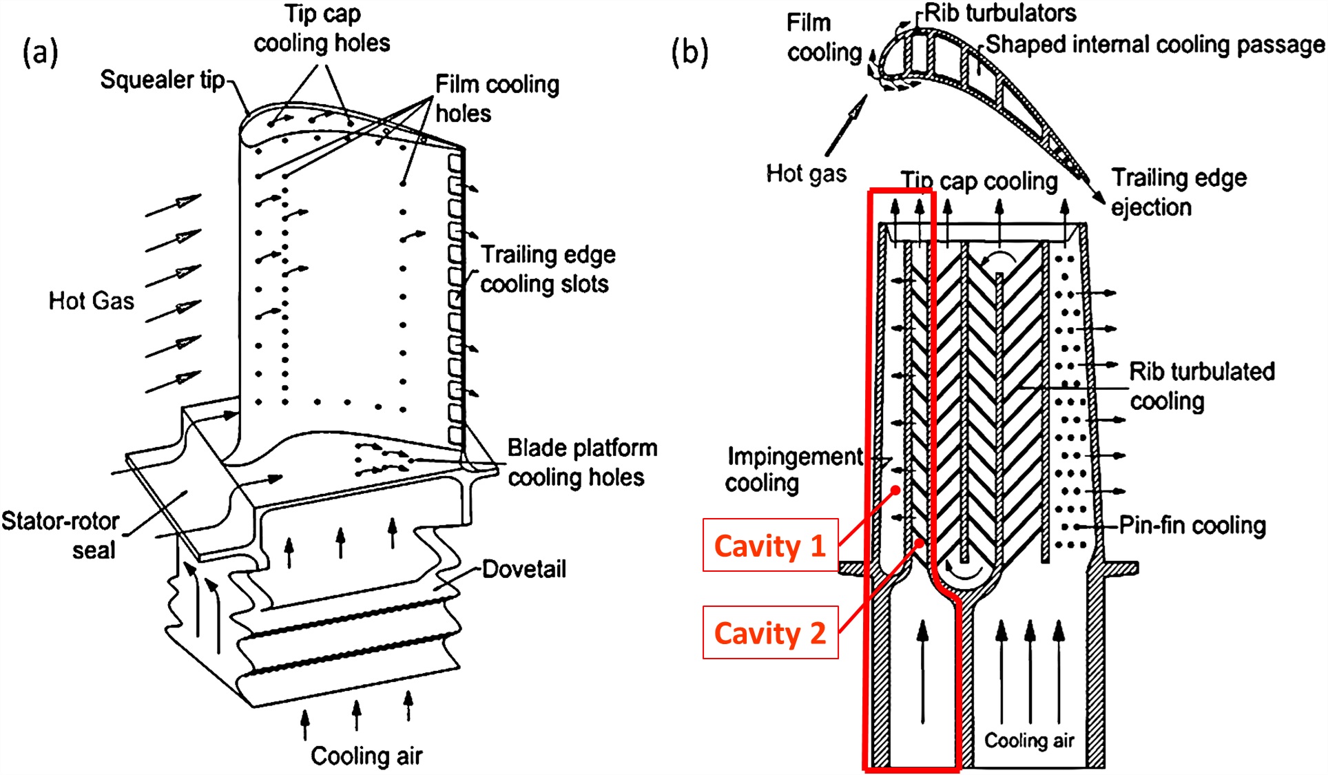
Figure 1.01: Turbine Blade Cooling Layout
- The LE passage is fed by cooling air from the compressor
- As the air travels radially outward it in Cavity 2, it will encounter turbulators on the cavity walls and exit the cavity through Crossover holes to Cavity 1 and Tip Cap holes into the Tip Squealer region.
- Three rows of ten film cooling holes exiting from Cavity 1 will cool the exterior of the Blade
Step 2: Load Blade Picture
- Right click on background and select Insert image
- Browse to image location and select open
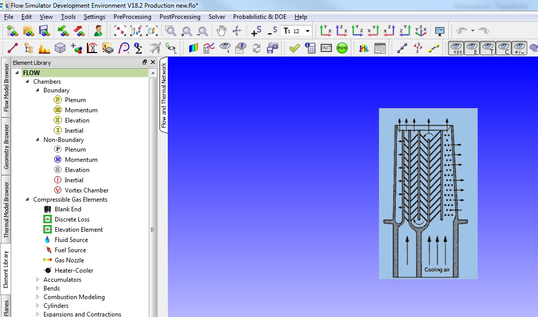
Figure 1.02: Loaded image on default background
- Go to settings → User Settings and the drop-down menu select Flow Simulator Default (This will turn your background blue)
- Exit the user settings and right click on the background and select change background color. In the window that pops up, select Pick Screen Color and click on the background of the blade image. Click OK. This should turn the background of flow simulator the same as that of the image.
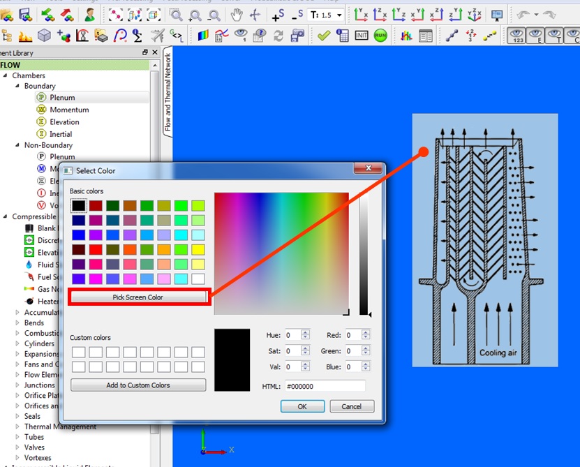
Figure 1.03: Adjusting Flow Simulator background
- Right click on the background and select Change text color. Set it to yellow (optional)
- It is easier to build a model on an image that is in the right location and has the
right scale. Adjust the image so that the base of the blade is located at a radius
(Y-Coordinate) of 10 and the tip of the blade is located at a radius of 13.
- Right click on the background and enable Selectable image in order to resize it using Ctrl + Left click on the corners
- Right lick on the image and select translate and use the menu to position the image in the right location, using the location readout at the bottom
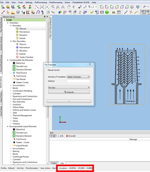
Figure 1.04: Adjusting image location
Step 3: Building Model
- Plan model setup based on what is known about the geometry
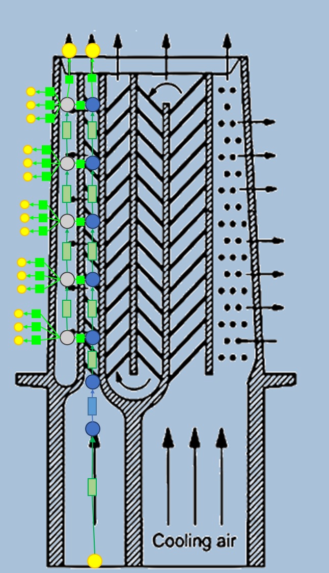
Figure 1.05: Sketch/Outline of model
- Set up the inlet and outlet boundary plenums by clicking and dragging to the following locations
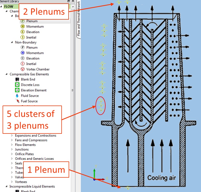
Figure 1.06: Boundary Plenum locations
- Set the inlet Plenum at the base of the blade to a Static Pressure of 800 Psi and Relative Total Temperature to 1000 F
- Set the two Plenums at the tip to pressure of 650 Psi and temperature of 2000 F
- Set the 5 clusters as shown in Figure 1.07 (to represent the Suction Side, Leading Edge, and Pressure Side of the showerhead film holes)
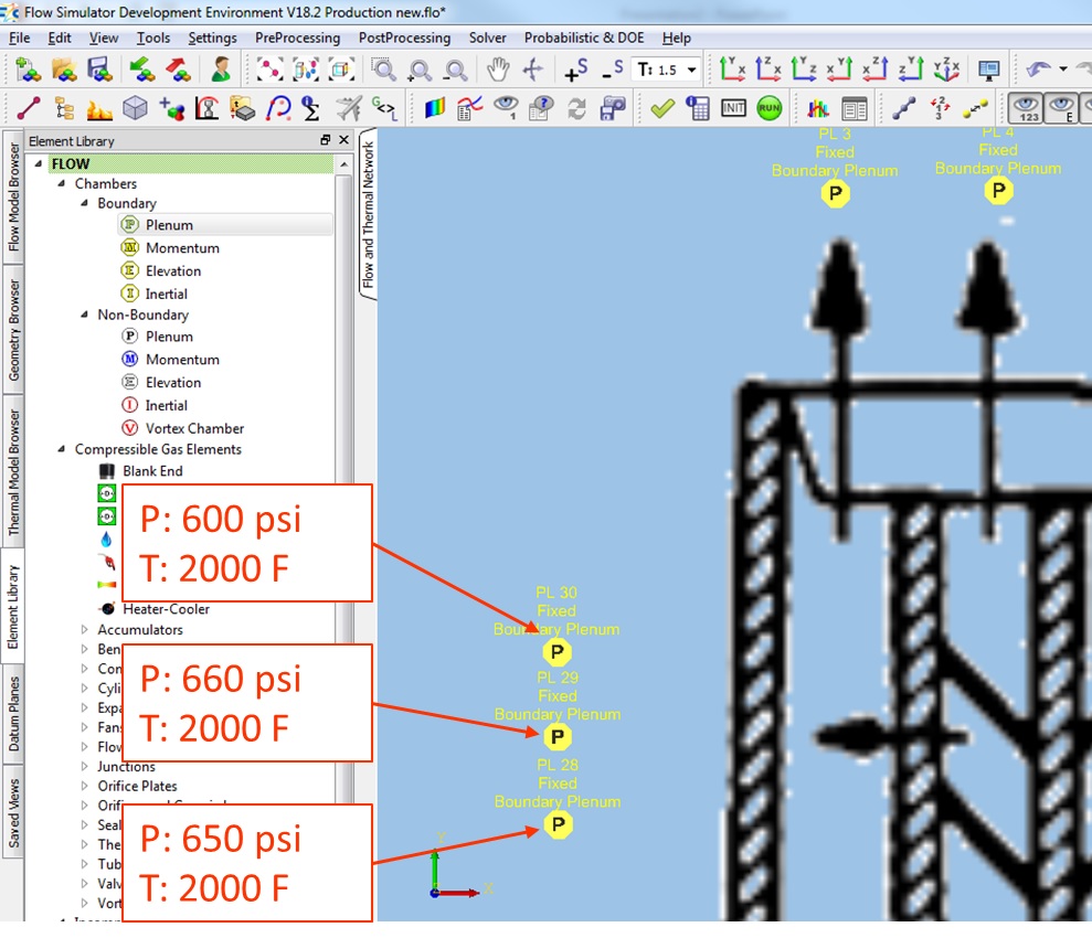
Figure 1.07: Boundary Conditions for Leading Edge setup
- Click and drag non-boundary momentum and plenum chambers to the location illustrated in figure 1.05
- Go to Solver → Analysis Setup → Reference Conditions and set the Steady-State Shaft
#1 Rotor Speed to 15000 RPM. Save
- Due to the rotating nature of the blade, the user will have to account for the pressure and temperature rise from the pumping created by the rotation, by enabling Chamber Swirl and specifying a Rotor Index for the elements.
- Select the momentum chambers and set the Chamber Swirl and Rotor Index as shown in figure 1.08
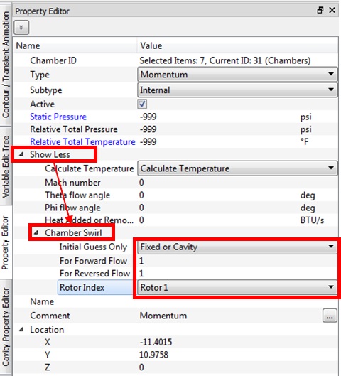
Figure 1.08: Swirl setup: non-boundary chambers
- Set up the Chamber Swirl and Rotor Index the same way for the non-boundary plenum chambers
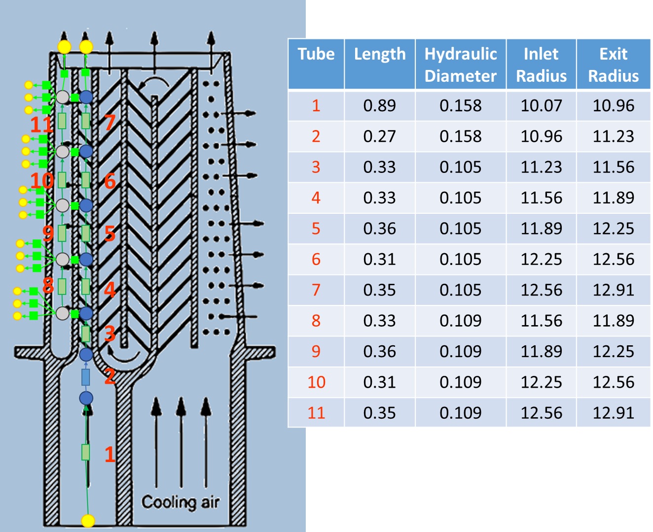
Figure 1.09: Tube Element Locations
- Place Simple Rotating tubes at the locations 1, 3-11 in figure 1.09 and a Standard tube at location 2
- Use the table on figure 1.09 to fill out the length, Hydraulic Diameter, and inlet and outlet radius for the Simple Rotating tubes
- At location 2, set up the standard tube as shown in figure 1.10
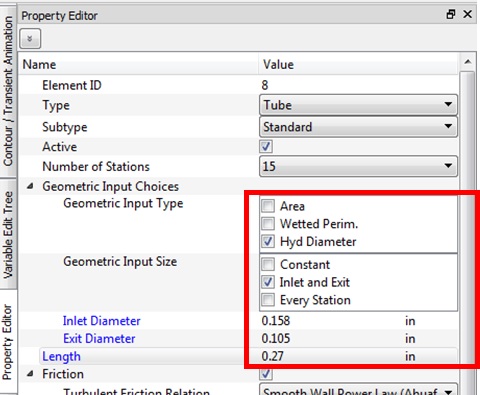
Figure 1.10: Location 2 Tube Element Set-up
- Set rotor index to “Rotor 1” for all tube elements and enter inlet and exit radius for the standard tube at location 2
- Set Advanced Options → Element Orientation → Element Inlet Orientation to “Radially
Outward” for all tube elements.
- This is to account for the flow making a turn to pass through the crossover holes and film holes because of the axial orientation in the elements representing those features
- Set Advanced Options → Heat Addition → Wall Temperature to 1100 F for all tube elements
- Set Friction → Friction Multiplier → Multiplier for Friction Losses to 4.5 on
locations 3-7 to model turbulators
- Applying a multiplier for Friction Losses allows the user to account for the losses due to turbulators without explicitly modeling them using a “Turbulated Passage” element
- Create Conventional Orifice elements at locations 1-7 in figure 1.11
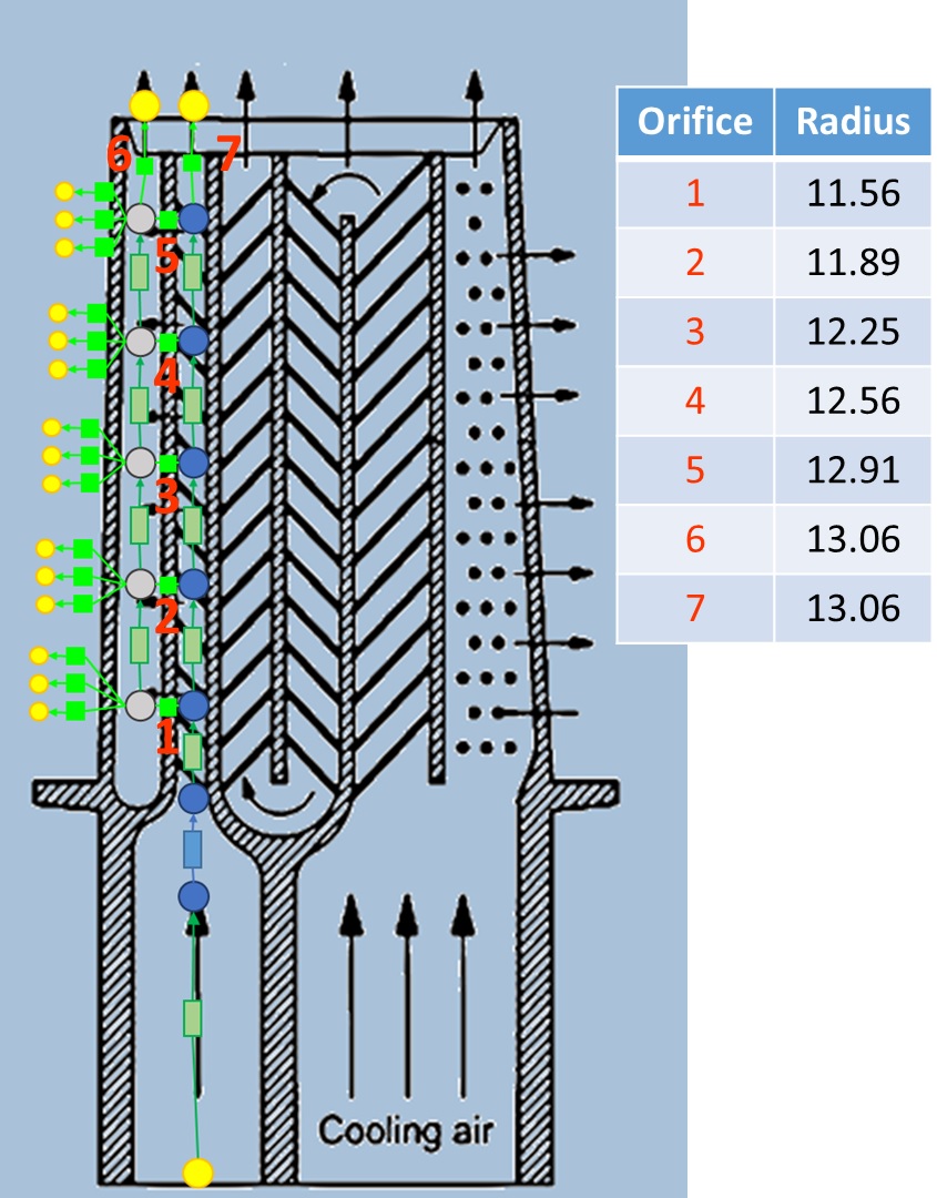
Figure 1.11: Conventional Orifice Element Locations
- Assign a diameter of 0.1 in and a Cd of 0.8 to Elements at locations 1-5
- Assign a diameter of 0.05 in and a Cd of 0.8 to Elements at locations 6 and 7
- Set element orientation to “Radially Outward” for Elements at locations 6 and 7, and leave the rest as Axial
- Set rotor index to “Rotor 1” for all Conventional Orifice Elements and use the table in figure 1.11 to assign a radius
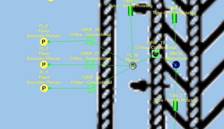
Figure 1.12: Film Hole Orifice Element Clusters
- Connect the plenums to the cluster of boundary plenums using Conventional Orifice elements to model the film holes exiting the blade near the Leading Edge as shown in figure 1.12
- Set Diameter to 0.02 in and Cd to 0.8 for all film hole Conventional Orifice elements
- Set Element Multiplicity Factor → No. of Streams Entering and Leaving to 2 for all
film hole Conventional Orifice elements
- The Element Multiplicity Factor allows for the use of a single element to represent several passages (in this case, 2 film holes per element)
- Set Rotor Index to “Rotor 1” for all film hole Conventional Orifice elements
- Set Radius for all 3 Conventional Orifice elements in each cluster the same as the connected Orifice element from figure 1.11
Step 4: Check Model and Run
- Select checkmark icon from the top toolbar
 to check the model for warnings/errors.
- An error should populate stating that the internal chamber has not been initialized
- Select the initialization icon from the toolbar
 , and pick Start. Accept values once flow solver has
converged.
, and pick Start. Accept values once flow solver has
converged. - Select run icon from toolbar
 . Run Flow Simulator.
Step 5: Post-process
- Results file (*.res) should automatically be loaded into GUI. If not, it can be selected via File → Load Result File
- By default, both chamber and elemental results are displayed in the graphical workspace.
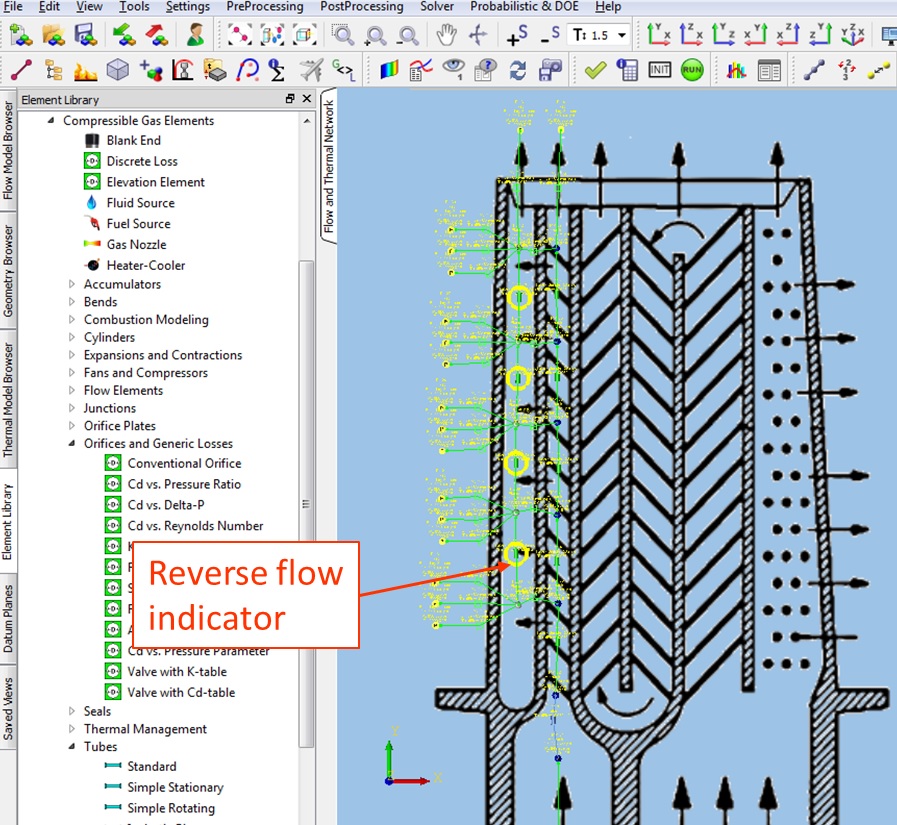
Figure 1.13: Results after model converges
- Select the Contour icon
 from the toolbar to open the Contour/Transient Animation tab and choose “Total
Pressure” from the first dropdown menu and “Result Data” from the second dropdown
menu and click Colorize.
from the toolbar to open the Contour/Transient Animation tab and choose “Total
Pressure” from the first dropdown menu and “Result Data” from the second dropdown
menu and click Colorize. - This displays a contour on the model that enables the user to visualize the pressures, as seen in figure 1.14
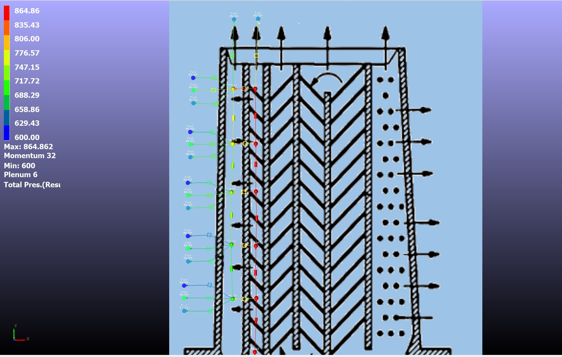
Figure 1.14: Contour plot of total pressure (Settings → User Settings allows customization of Stream Line Thickness)