Tutorial 12: Integrated Flow & Thermal Network Model
Purpose/Objective
This exercise will walk the user through building an integrated thermal network for a simple piping system. The user will learn how to:
- Edit thermal chamber properties
- Edit thermal element properties
- Couple the flow and thermal networks.
- Check the model
- Run the model
- Post-process the model
- Thermal Network: Convection and Conduction
- Fluid: Air
Step 1: Examine geometry and create plan
- The user will be creating a thermal model of a simple tube and boundary conditions
shown in Figure 1.01.
- The scope of this example will be focused on the thermal portion of model building and will start from an already existing flow model.
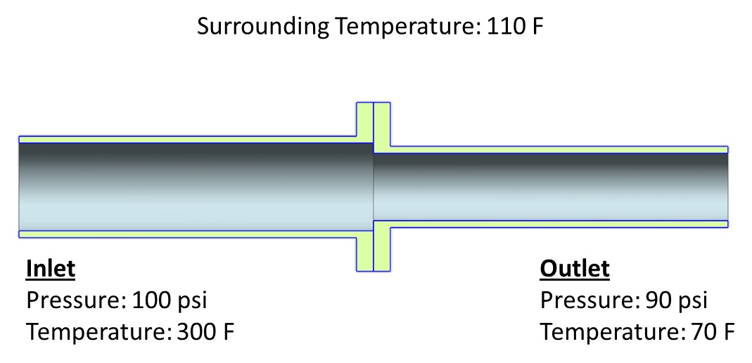
Figure 1.01: Pipe geometry and boundary conditions
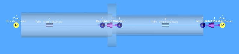
Figure 1.02: Existing flow model to be used a starting point for the thermal model
- The model consists of a straight pipe mated to a smaller diameter straight pipe with a flange.
- To capture the heat transfer through the pipe walls, the user will be using thermal nodes and convector and conductor elements
Step 2: Open Starting Model
- Go to File → Open
- Browse to starting model location and open: Ex_12_starting_model.flo
Step 3: Building Model
- Plan model setup based on what is known about the geometry
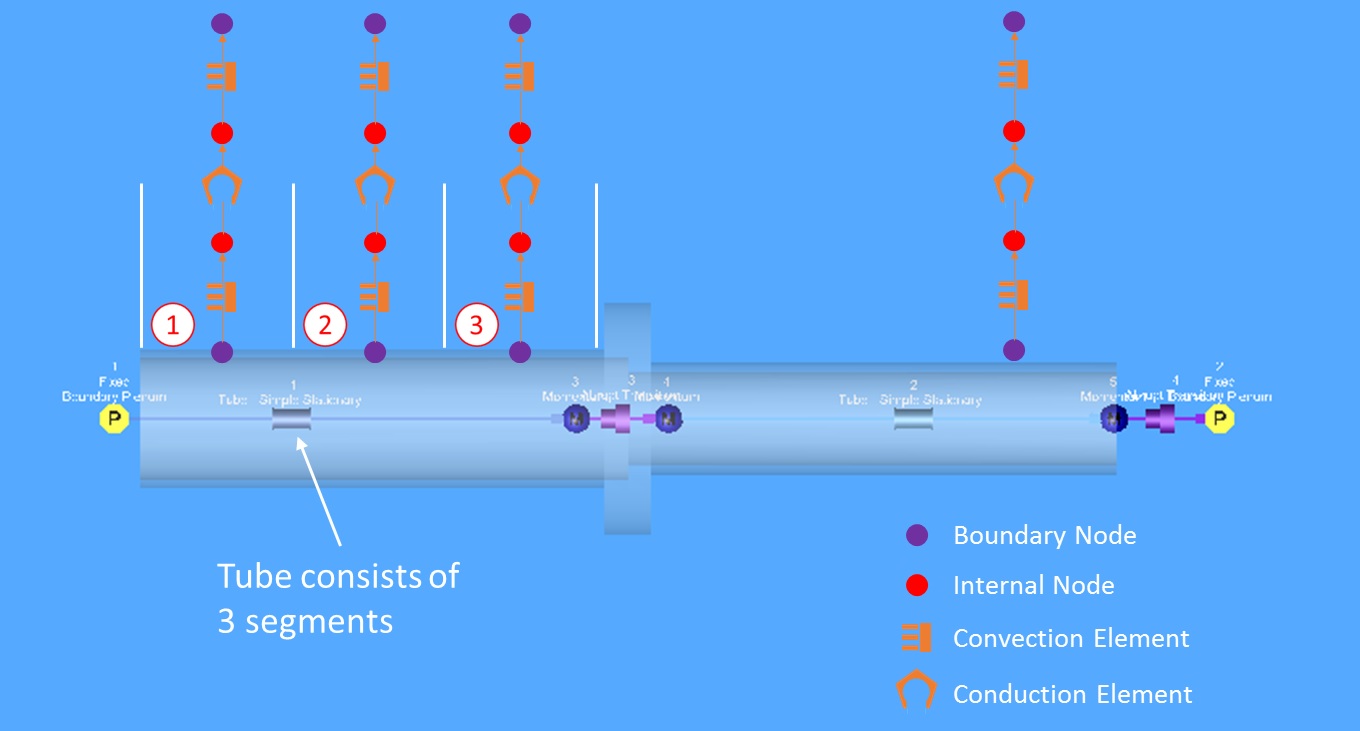
Figure 1.03: Sketch/Outline of building thermal model on top of flow model
- The flow in the larger pipe (left) is being modeled by a tube element that has 4 stations, which translates to 3 segments. Heat transfer for that pipe will be coupled to segments in the tube element, which will allow for thermal convection to use HTCs directly from the tube. The thermal model on the smaller pipe will demonstrate a different method of coupling the flow and thermal network. The momentum chamber at the end of the pipe will be coupled to the thermal network.
- Drag and drop the two Thermal Boundary TNodes at the locations shown for thermal
circuit 1 in Figure 1.03 (purple circles)
- In the node representing the pipe wall, set Associated Item Type to
Element
- Set Associated Item ID to 1
- Set Associated Segment to 1
- In the node further from the pipe wall, set Node Temperature to 110 F
- In the node representing the pipe wall, set Associated Item Type to
Element
- Drag and drop the two Thermal Internal Tnodes shown in Figure 1.03 (red circles) to
their locations in circuit 1
- For the internal node close to the pipe, set Associated Item Type to
Element
- Under Coupling Method with Flow Network, check Send Wall Temperature to Flow Network
- Set Associated Item ID to 1, Associated Segment to 1, and Associated Circumferential Wall Segment to 1
- Set Mass Type to Arithmetic Node
- For the internal node further from the pipe, set Node Temperature to 110 F
(this is an initial temperature guess to help the model with
initialization)
- Set Mass Type to Arithmetic Node
- For the internal node close to the pipe, set Associated Item Type to
Element
- Connect the internal nodes to the boundary condition nodes with Convector
Elements
 and connect the two internal
nodes with a Conductor Element
and connect the two internal
nodes with a Conductor Element  (Figure 1.04)
- For the convection element closer to the pipe, set Surface Area to 6.9
in^2
- Under Heat Transfer Coefficient Calculation Method, check “Use Element’s HTC”
- For the convection element further from the pipe, set Surface Area to 7.3
in^2
- Set Heat Transfer Coefficient to 15 BTU/hr*ft^2*F
- For the conduction element, change Conductor Type to Radial
- Under Conductivity Method, check FI Solid Properties Library
- Set Length to 1.7 in, InnerRadius to 0.65 in, and OuterRadius to 0.7
in
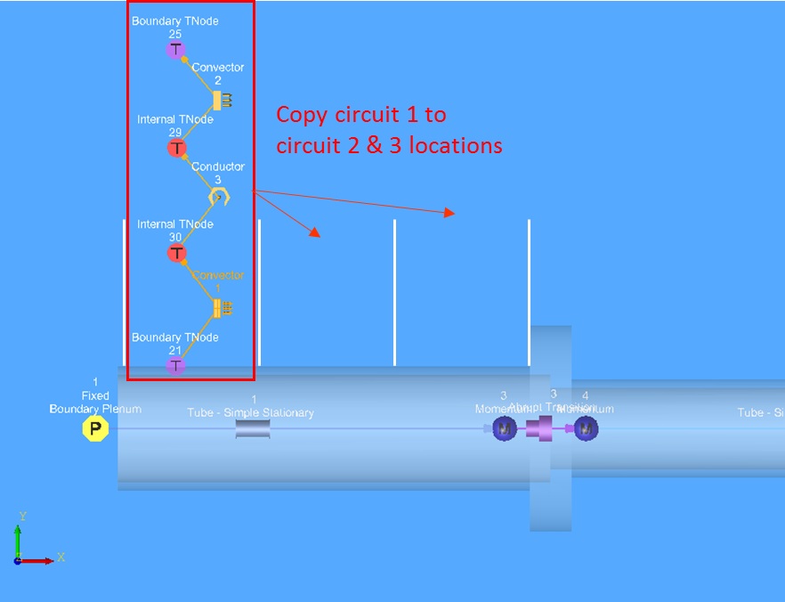
Figure 1.04: Thermal circuit set-up
- For the convection element closer to the pipe, set Surface Area to 6.9
in^2
- Now that circuit 1 setup is complete, it can be copied to the circuit 2 & 3
locations
- Select all thermal nodes and elements, press Ctrl+C, and click to paste
- Select the new set of nodes and elements and use translate (right click on nodes/elements → translate) to adjust their location
- For thermal circuit 2
- Change Associated Segment from 1 to 2 for the internal node and boundary node located closer to the pipe
- The Segment ID for the Convection element closer to the pipe will automatically change from 1 to 2
- For thermal circuit 3
- Change Associated Segment from 1 to 3 for the internal node and boundary node located closer to the pipe
- The Segment ID for the Convection element closer to the pipe will
automatically change from 1 to 3
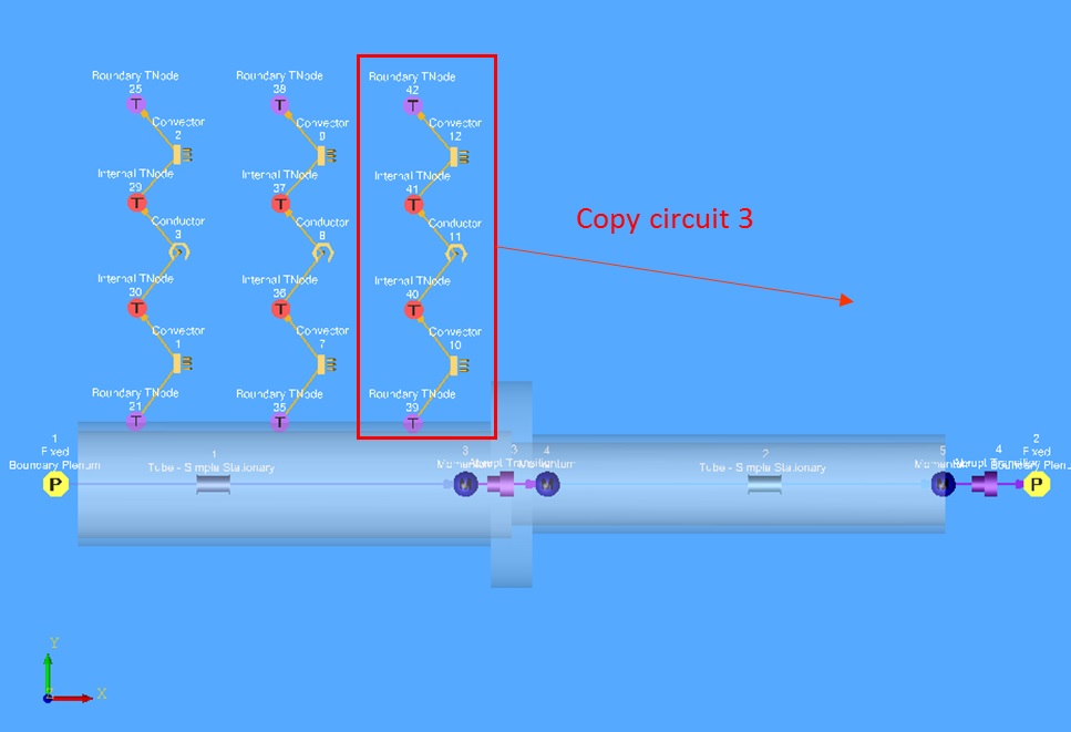
Figure 1.05: Smaller pipe thermal circuit set-up
- Copy circuit 3 via the method used earlier, and place it near the exit of the smaller pipe
- For the Boundary Node closer to the pipe
- Change Associated Item Type from Element to Chamber
- Set Associated Item ID to 5
- For the Internal Node close to the pipe
- Change Associated Item Type to None
- Set Node Temperature to 110 F as an initial guess for the solver
- For the Convection Element close to the pipe
- Set Surface Area to 15.7 in^2
- Change Heat Transfer Coefficient Calculation Method from Use Element’s HTC to Fixed HTC
- Set Heat Transfer Coefficient to 50 BTU/hr*ft^2*F
- For the Conduction Element
- Set InnerRadius to 0.5 in and OuterRadius to 0.6 in
- For the Convection Element further from the pipe
- Set Surface Area to 18.8 in^2
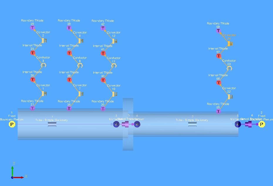
Figure 1.06: Finished model thermal circuit set-up
- Set Surface Area to 18.8 in^2
Step 4: Check Model and Run
- Select checkmark icon from the top toolbar
 to check the model for warnings/errors.
- An error should populate stating that the internal chamber has not been initialized
- Another error should mention the Analysis Type = Steady State Flow
- Select the initialization icon from the toolbar
 , and pick Start. Accept values once flow
solver has converged.
, and pick Start. Accept values once flow
solver has converged. - Analysis Setup → Analysis Type = Steady State Flow + Steady State Thermal
- Select run icon from toolbar
 . Run Flow Simulator.
Step 5: Post-process
- Results file (*.res) should automatically be loaded into GUI. If not, it can be selected via File → Load Result File
- By default, both flow chamber and flow elemental results are displayed in the graphical workspace.
- Node temperature display may have to be enabled in Settings → Display Options → Thermal Results → Nodal Temperature
-
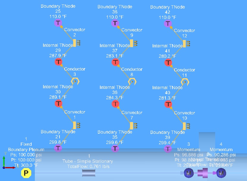
Figure 1.07: Thermal results after running model
- Figure 1.07 shows the fluid temperatures represented by the purple thermal boundary condition nodes and the wall temperatures represented by the red thermal internal nodes.
- In this example it can be observed that the pipe wall temperatures are primarily driven by the internal fluid because both internal and external wall temperatures are much closer to the internal fluid than the external ambient temperatures