Tutorial 14: 2D Conduction Problem - Thermal Network Model
Purpose/Objective
This exercise will walk the user through building an integrated 2D thermal network for Fire Clay Brick. The user will learn how to:
- Set Unit system
- Creation of custom solid material (Fire clay brick)
- Edit thermal chamber properties
- Edit thermal element properties
- Check the model
- Run the model
- Post-process the model
- Thermal Network: Convection and Conduction
- Material: Custom Material (Fire clay brick)
Problem Statement
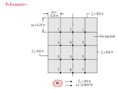
A large industrial furnace is supported on a long column of fireclay brick, which is 1m by 1 m on a side. During steady-state operation, installation is such that three surfaces of the column are maintained at 500 K while the remaining surface is exposed to an airstream for which T=300 K and h=10 W/m2 K. Using a grid of x=y=0.25 m, determine the two-dimensional temperature distribution in the column and the heat rate to the airstream per unit length of column.
Step 1: Set Unit System
- Go to Settings → Unit Maintenance
- Set SI as a preferred unit system by selecting SI under “Unit Set” Window
and then clicking
 button.
 - Check all the unit system are consistent as per the inputs from the problem
statement.
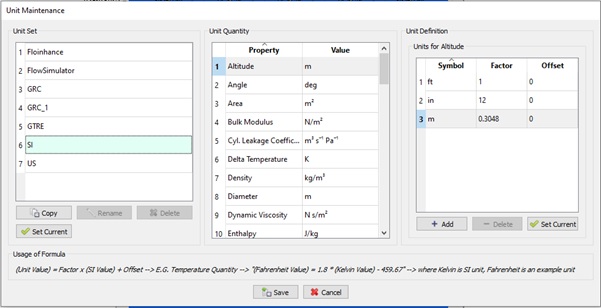
Figure 1.01: Unit System configuration
- Set SI as a preferred unit system by selecting SI under “Unit Set” Window
and then clicking
- We will be using unit system for Heat transfer co-efficient as W/m2 C instead of W/m2 K as conversion factor between these unit system is 1.0.
- Click
 to set it as default unit
system.
to set it as default unit
system.
Step 2: Creation of custom solid material (Fire clay brick)
- Go to PreProcessing → Material Manager
- Under Solid Window click
 . A popup “Material Editor” window will
open.
. A popup “Material Editor” window will
open.- Provide Material name “FireClayBrick” inside Material Name Box.
- Activate “Specific Heat” & Thermal Conductivity”. Change the unit system as shown in Figure 1.02 below if required.
- Enter 18672810 as value inside “Specific Heat” row.
- Enter 25 as value inside “Thermal Conductivity” row.
- Click Save.
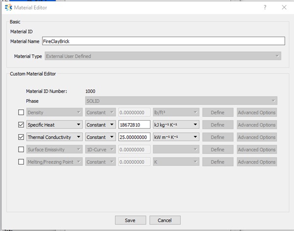
Figure 1.02: Material Editor Configuration
Step 3: Building Model
- Plan model setup based on what is known about the geometry.
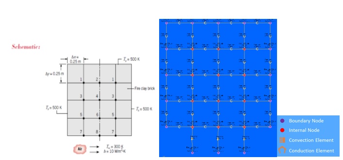
Figure 1.03: Sketch/Outline of building thermal model on top of flow model
- The entire fireclay brick will be modelled by 2D grid of thermal chambers (Boundary/Internal) & Conductor Element. Top, left & right thermal chambers Boundary temperature will be 500K. Internal & Bottom chambers will be modelled as Internal chambers as those values are unknown. These will be calculated by solver using Energy Equation. Bottom Fluid air chambers are modelled as thermal chambers with fixed Boundary temperature as 300K. These fluid chambers will be connected to bottom of fireclay brick using Convection Element.
- Drag and drop
 &
&  to create grid as shown in the Figure
1.03.
to create grid as shown in the Figure
1.03. - Drag and drop Convector Elements
 and Conductor Element
  to connect Boundary TNode & Internal
TNode as shown in the Figure 1.04.
to connect Boundary TNode & Internal
TNode as shown in the Figure 1.04.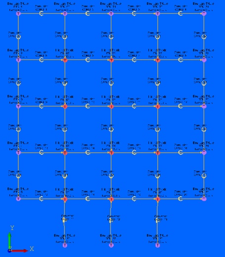
Figure 1.04: Construction of Thermal Network
- Provide thermal boundary condition for thermal chambers/nodes as shown in Figure
1.05
- Select top, left & right Boundary TNodes of Brick Clay
- Inside Property Editor under Node Temperature enter value as 500K
- Select Boundary TNodes of Fluid stream
- Inside Property Editor under Node Temperature enter value as 300K
- All other Internal TNodes enter Node Temperature value as 500K (initial guess)
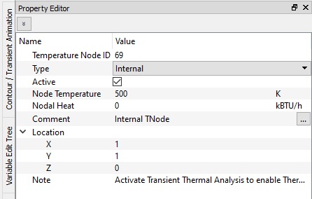
Figure 1.05: Thermal TNode Chambers set-up
- Select top, left & right Boundary TNodes of Brick Clay
- Provide thermal boundary condition for conductor as shown in Figure 1.06
- Select all internal thermal conductor
- Change Conductor Type to “Simple”.
- Change Material List as “FireClayBrick”.
- Enter Cross-Section Area as 387.5 in^2
- Enter thickness as 9.842525 in.
- Select all external thermal conductor
- Change Conductor Type to “Simple”.
- Change Material List as “FireClayBrick”.
- Enter Cross-Section Area as 193.75 in^2
- Enter thickness as 9.842525 in.
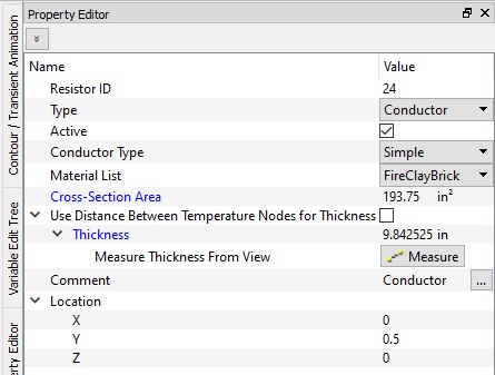
Figure 1.06: Conductor circuit set-up
- Select all internal thermal conductor
- Provide thermal boundary condition for convection as shown in Figure 1.07
- Select all thermal convectors
- Change “HTC Relation” to “Fixed HTC”
- Enter “Heat Transfer Coefficient” as 10W/m^2C
- Enter “Surface Area” as 387.5 in^2
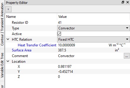
Figure 1.07: Convector circuit set-up
- Select all thermal convectors
- Click
 to save the model.
Step 4: Check Model and Run
- Select checkmark icon from the top toolbar
 to check the model for warnings/errors.
- An error should mention the Analysis Type = Steady State Flow
- Select the initialization icon from the toolbar
 , and click Start. Accept values once flow
solver has converged.
, and click Start. Accept values once flow
solver has converged. - Analysis Setup → Analysis Type = Steady State Thermal
- Select run icon from toolbar
 . Run Flow Simulator.
Step 5: Post-process
- Results file (*.res) should automatically be loaded into GUI. If not, it can be selected via File → Load Result File
- By default, both thermal node and thermal elemental results are displayed in the graphical workspace.
- Node temperature display may have to be enabled in Settings → Display Options →
Thermal Results → Nodal Temperature
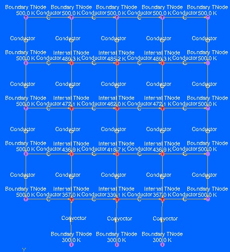
Figure 1.08: Thermal results after running model
- Figure 1.08 shows the internal metal temperature is represented by the red thermal boundary condition nodes
- User can also create plot contour as shown in Figure 1.09
- Go to PostProcessingà Contour / Transient Animation
- Select Mode as “Coloring”
- Choose “Total Temperature” & “Result Data” under Data Source
- Click “Colorize”. Click “Reset” to back to normal view.
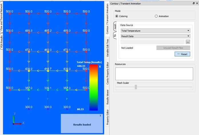
Figure 1.09: Total Temperature Contour plot