Geometric and Solution Adaption
SimSolid adaption tools and solution settings best practices.
SimSolid enables both geometric and solution adaptations, with various settings available to fine-tune these adjustments. All adaptation controls can be found within the Solution Settings window. Options include global and global+local objectives, as well as a custom objective with various controls to achieve the desired solution accuracy. The following information explains how each objective functions and provides guidance on which option to select for obtaining high-fidelity solutions in SimSolid.
These options are applicable to all analyses supported by SimSolid and can be customized or adjusted for each individual subcase.
Geometry Adaptation
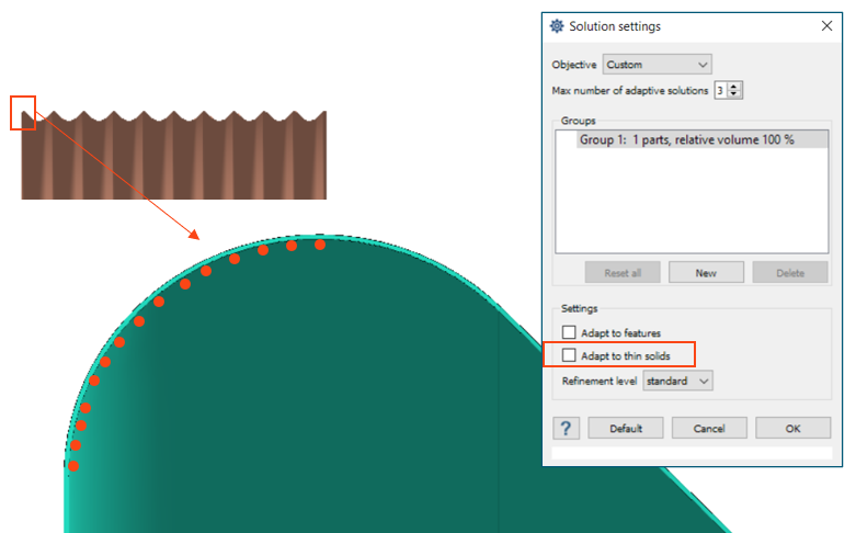
Adapt to Thin Solids
Adapt to Thin Solids is one of the key options for controlling geometry adaptation. For assemblies with thin-walled structures or parts exhibiting varying curvatures, it is strongly recommended to use this feature. It identifies areas with local curvatures and adapts for these geometric changes by introducing additional degrees of freedom. This ensures that geometric variations are accurately captured during the solution stage.
The figure below shows an example of a corrugated sheet. When Adapt to Thin Solids is activated, additional degrees of freedom are introduced along the curvature. For example, the red dots illustrate the locations of degrees of freedom with Adapt to Thin Solids applied. In the absence of this feature, there are generally fewer red dots, which results in lower resolution and often causes the structure to exhibit increased stiffness.
Groups
Groups also play a key role in geometry adaptation. The scale of a group influences the initial refinement level of the geometry decomposition, much like defining the global mesh parameter in traditional Finite Element (FE) analysis. For instance, if one part occupies 80% of the volume, it will dictate the initial refinement level for that assembly, potentially leading to insufficient refinement for other smaller components.
In traditional Finite Element (FE) analysis, it's common to increase mesh density for smaller, critical areas. Similarly, in SimSolid, it's important to create local groups to achieve appropriate refinement for smaller parts. This approach ensures that each component receives the necessary level of detail, improving the accuracy and reliability of the analysis.
The level of initial refinement can also be adjusted by modifying the refinement settings, which can be applied to individual groups, sets of parts, or the entire assembly.
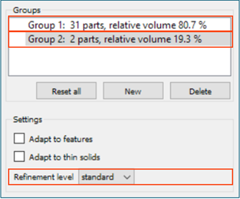
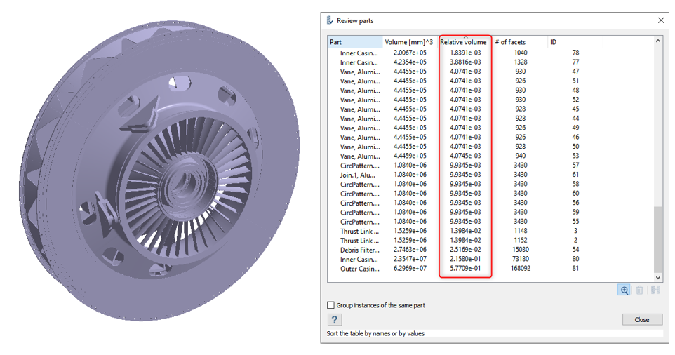
The Review Parts Assembly tool provides a comprehensive list of all parts in the assembly along with their relative volumes. Parts can be sorted by volume, organize them into local groups, and set the appropriate refinement levels. When creating local groups, ensure that parts of similar sizes are grouped together to avoid mixing different sizes within a single group.
The Global+Local objective in SimSolid automates the creation of local groups for parts of different sizes and applies the suitable geometry and solution adaptation settings. This automation simplifies the process, particularly for cases dealing with large assemblies, by minimizing the need for manual group creation.
Solution Adaption
In conventional finite element analysis (FE), the process usually ends after meshing the model and executing the analysis. SimSolid, on the other hand, incorporates an advanced feature called solution adaptation.
Adaptive Passes
As a multi-pass adaptive solver, SimSolid first conducts an analysis with an initial geometry adaptation. It then examines the results for errors and makes targeted adjustments by refining specific parts of the assembly or individual features—such as holes, constraints, or connections—by increasing the degrees of freedom. The solver then progresses through a series of passes as specified in the solution settings. This iterative approach enhances accuracy and ensures that critical areas receive detailed attention.
For the Global objective, SimSolid runs through 3 passes, while the Global+Local objective runs for 4 passes. It is generally advised not to exceed six passes; instead, creating local groups is recommended for further refinement. Increasing the number of passes can escalate the complexity and order of the function, which may not always be necessary.
Error Criteria
When running analyses, SimSolid performs a series of passes and evaluates various error types at each stage.
- Global Energy Measure identifies regions of higher strain energy within the assembly and adapts locally to these areas to improve accuracy.
- Displacement Error focuses on boundary regions—such
as constraints or connection points. For instance, in the analysis of a
cantilever beam, SimSolid starts by introducing
a degree of freedom at the support region and assesses errors at the end of
each pass. If the boundary conditions are not fully met, additional degrees
of freedom are added, and this process continues through the specified
number of passes until the boundary conditions are satisfied. Similar method
is applied to connections.
Figure 6. 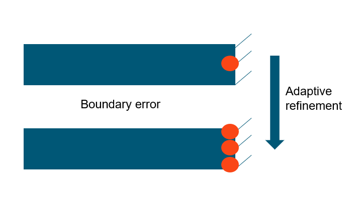
Avoid using single-line connections and discrete points because they can introduce instabilities, especially when performing a higher number of passes. Discrete points can create discontinuities in the model, leading to localized stress concentrations that tend to increase with each pass. This can result in inaccurate stress predictions and potential convergence issues. To ensure more stable and reliable results, use continuous connections.Figure 7. Discrete connections (left) and well-defined connections (right) 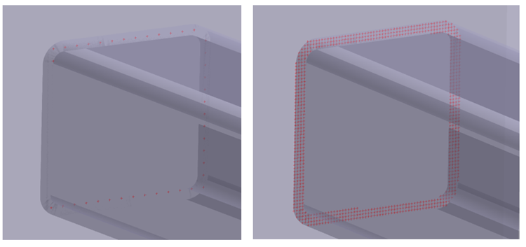
- Traction Error management is facilitated by enabling
the Adapt to Features option. Global+Local objective utilizes this feature
to enhance accuracy. Traction adaptation can be applied to specific parts,
groups of parts, or the entire assembly. For detailed stress data, always
enable Adapt to Features. SimSolid identifies
regions with significant stress gradients and performs localized adaptations
by increasing degrees of freedom. By default, SimSolid already adapts to features such as holes.
With Adapt to Features enabled, the solver will also address traction errors
throughout the entire assembly, including complex features like fillets and
torus faces, ensuring that these areas receive appropriate refinement and
adjustment.
Figure 8. 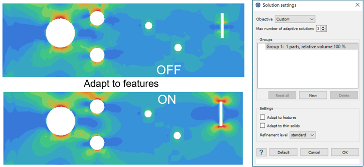
The image at the top shows the results with "Adapt to Features" turned off. By default, SimSolid adapts locally around holes and predicts stress concentrations in these areas effectively. However, it may not accurately capture stresses around geometries like rectangular slots, which can be singularity zones due to sharp corners. Consequently, the stress predictions might differ from those obtained with a more refined finite element (FE) setup.
When Adapt to Features is enabled, the stress pattern improves significantly. The adaptation process better captures the stress concentration around the rectangular slot and provides a better overall stress distribution.
Traction error is determined based on the maximum stress observed in the assembly. SimSolid identifies traction errors in areas where stress levels are within a certain percentage of this maximum stress and adapts locally in these regions. Sharp corners, discrete connections, and boundary conditions applied to points—often sources of singularity—can lead to regions with exaggerated stress concentrations. These areas may cause the solver to aggressively adapt, potentially skewing results. Therefore, it is advisable to avoid such problematic configurations.
For well-defined problems, enable Adapt to Features to achieve high-fidelity stress predictions.
Examples
- Sharp Corners and Geometric Singularities: The
following example demonstrates how sharp corners can affect stress distribution.
- Model with sharp corners: This image displays
a model with sharp corners. The presence of these sharp features
leads to localized stress concentrations, which can cause inaccurate
stress predictions.
Figure 9. 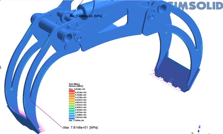
- Model without sharp corners: This image shows
the same model with the sharp corners smoothed or replaced with
fillets. The stress distribution in this case is much more even,
reflecting a more realistic pattern.
Figure 10. 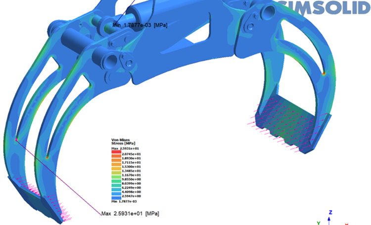
This comparison emphasizes the importance of addressing sharp corners in your design. By rounding or smoothing these features, you can achieve a more accurate stress distribution and improve the overall reliability of your analysis.
- Model with sharp corners: This image displays
a model with sharp corners. The presence of these sharp features
leads to localized stress concentrations, which can cause inaccurate
stress predictions.
- Discrete connections: The following example
highlights how discrete connections can influence stress distribution.
- Model with discrete connections: This image
shows discrete connection points between the vertical plate and the
horizontal square tube. Such discrete connections can cause
localized stress concentrations, which may lead to inaccurate stress
predictions.
Figure 11. 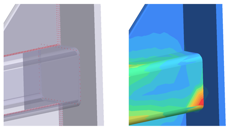
- Model with well-defined connections: This
image demonstrates that increasing the resolution of the connections
helps to mitigate singularity regions, leading to a more accurate
and evenly distributed stress profile.
Figure 12. 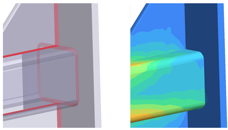
- Model with discrete connections: This image
shows discrete connection points between the vertical plate and the
horizontal square tube. Such discrete connections can cause
localized stress concentrations, which may lead to inaccurate stress
predictions.
- Bolt contact connections with pretension: The
following example illustrates the impact of improper contact conditions.
- Model with bonded contact at the shank: This
shows bolts with bonded contacts at the shank region. Here, improper
contact conditions lead to excessive adaptation around the bolt
areas, resulting in high stress concentrations.
Figure 13. 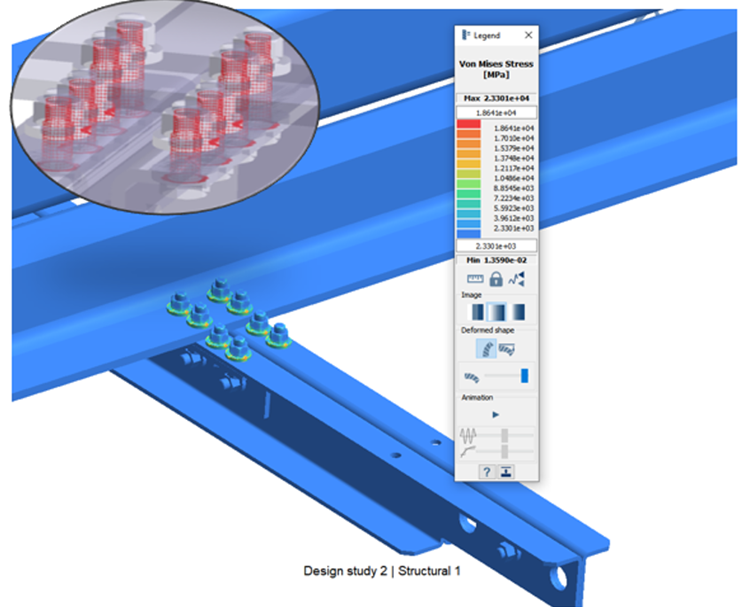
- Model with sliding contact at the shank: This
shows bolts with properly defined sliding contacts. In this case,
the stress distribution is much more even, reflecting a more
accurate stress pattern.
Figure 14. 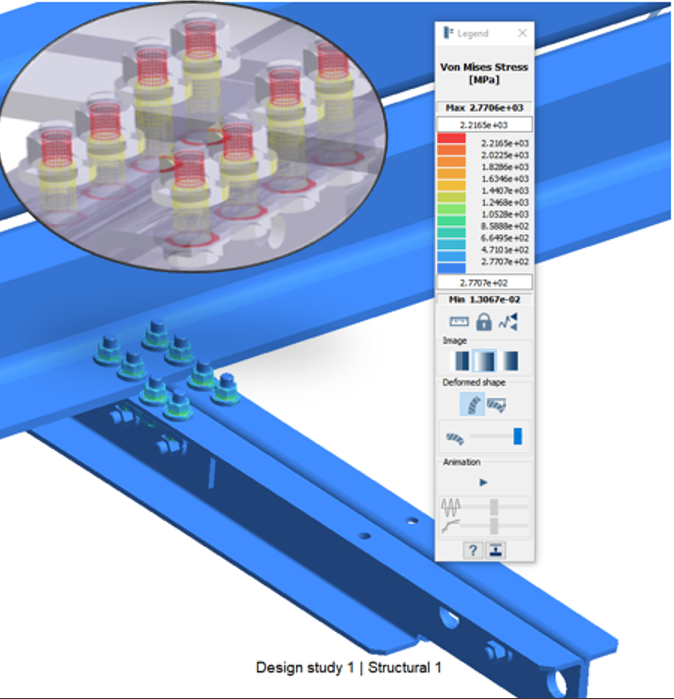
This example highlights the importance of using appropriate contact conditions. Ensuring the correct definition of contact types is crucial for resolving pretension, achieving accurate stress distributions and avoiding misleading results.
- Model with bonded contact at the shank: This
shows bolts with bonded contacts at the shank region. Here, improper
contact conditions lead to excessive adaptation around the bolt
areas, resulting in high stress concentrations.
Overall Guidelines
- Adapt to Features: Use this option to selectively increase degrees of freedom around small or intricate features, such as holes or fillets, to improve accuracy in stress analysis.
- Adapt to Thin Solids: Apply this setting to increase degrees of freedom around thin, curved parts, ensuring more precise results for these critical areas.
- Use Local Groups for:
- High-Fidelity Stresses: Detailed stress analysis at specific locations within the assembly is required.
- Scale Differences: There is a significant difference in the scale of various parts in the assembly.
- Mixed Materials: The assembly includes a combination of stiffer and softer materials, requiring localized refinement to capture interactions accurately.