Using Solution
![]()
Introduction
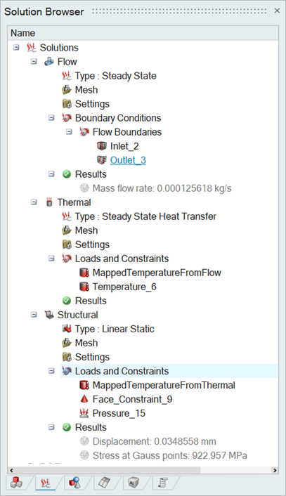
SimLab enables users to solve complex problems involving multiple physical parameters. DOE allows to study the impact of those parameters. Users can select a solution to define DOE. SimLab automatically picks up the parameters used in the solution. These parameters include initial condition, boundary condition, material properties, and other relevant input.
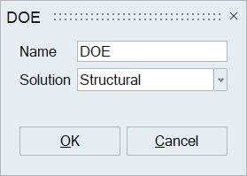
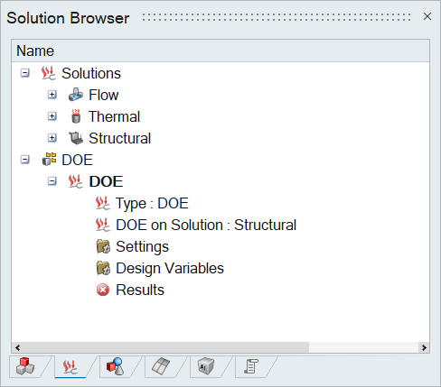
Select a solution to set up DOE. This will create a DOE solution in the solution browser. That will guide to setup and execute experiments.
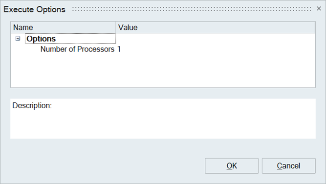
The “Execute Options” in RMB click on “Settings” allows to define the number of processors to run experiments in parallel.
Double-clicking “Design Variables” in the DOE solution will list all the parameters that are associated with the solution and its coupled solutions. The “DOE” column in this table allows the user to select parameters that the user wants to include for experiments.
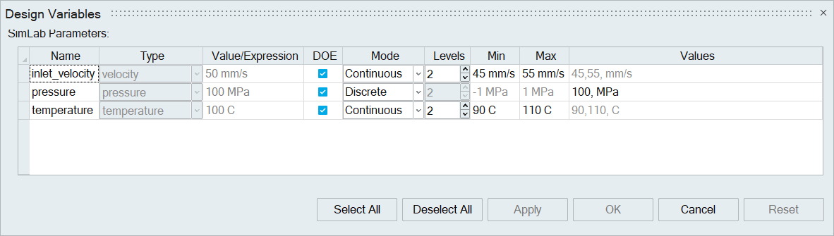
“Continuous” and “Discrete” are two different modes to define the parameter. “Continuous” mode allows the definition of range and number of levels in between. “Discrete” mode allows the definition of multiple discrete values.
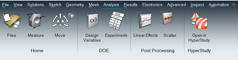
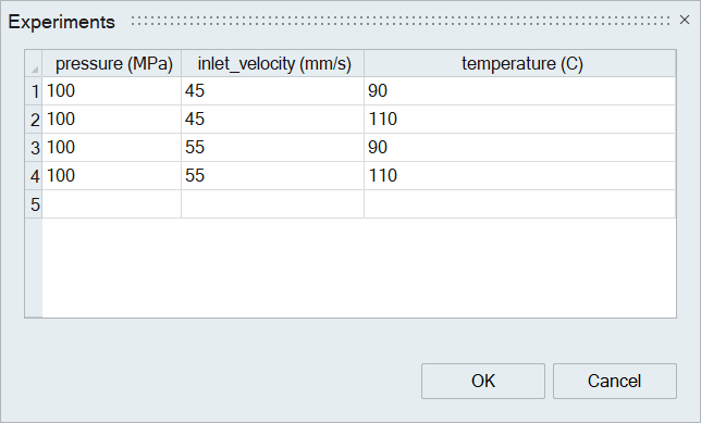
The experiments table can be displayed by clicking on “Experiments” in the Analysis ribbon. This will show a table with a set of experiments created based on the parameters defined. This table allows users to add/remove experiments and change the parameter value.
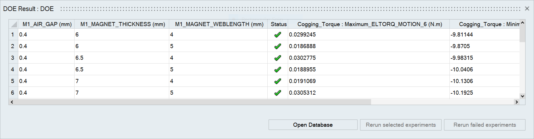
The “Update” option in RMB click on “Results” in the DOE solution start executing the experiments. The status of each experiment will be updated in the DOE table. User can select a maximum of 4 experiments by selecting the row to open the database by clicking “Open Database”.
To visualize data, users can select multiple experiments from the table by selecting rows and click “Plot Scalars and Vectors.” This option displays both parameter and response values from the selected experiments as plots.
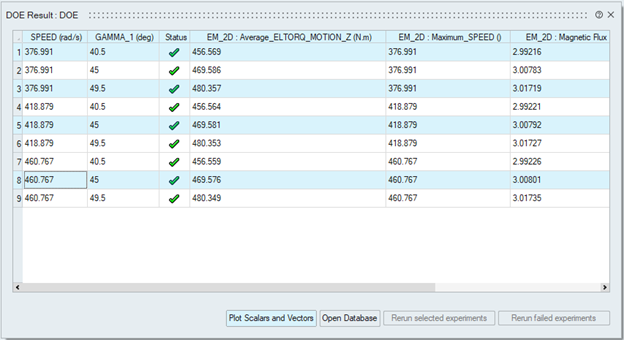
Although the parameters and responses are shown as scalar values in the table, some responses may originate from time-dependent results. For example, the response average_eltorq_motion_z is a time-dependent quantity. When such responses are included in the DOE table, their corresponding time variation will also be shown in the plot.
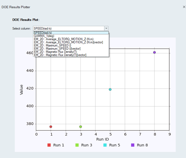
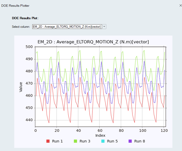
After selecting the desired experiments and clicking “Plot Scalars and Vectors” the DOE Results Plotter will appear on the right side. A dropdown menu in the plotter allows users to select specific parameters or responses from the DOE results. Time-dependent responses, if available, will also appear in this dropdown and can be plotted as shown in the figure below.
Exporting as JSON Files
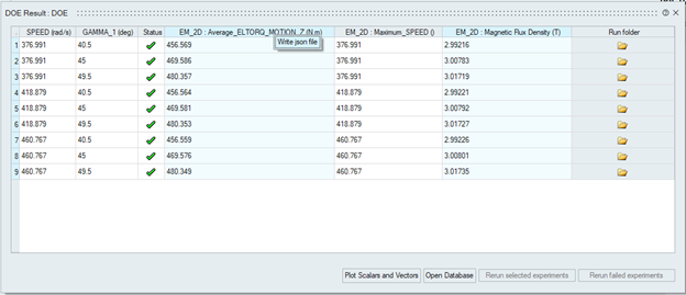
From the DOE Results Table, users can export the parameters or responses of each experiment in the form of a JSON file, which can then be used for Physics AI training.
The Key Performance Indicators (KPIs) must be provided through .json files, in addition to the solver result files (for example, .h3d, .odb, etc.) or solver input decks (for example, .fem, .rad, etc.). These files should be placed in the same subdirectory and share the same name.
To export results as a JSON file:
- Select the columns you want to export from the DOE Results Table.
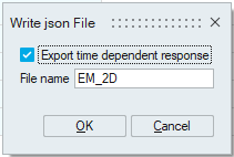
- Right-click and choose “Write JSON File”.
- Enter a file name for the JSON export.
- (Optional) If any of the selected responses are time-dependent, check
the corresponding box to include their time history data.
- The JSON file will be generated in the same location as the result files for that experiment.
For more details on how JSON files are used in Physics AI workflows, refer to the following tutorials:
To use the DOE Plotter and JSON export features, ensure that the Base Solution is updated before executing the DOE solution so that the base solution responses are stored correctly.
If the DOE solution was solved using a previous version, time-dependent responses may not be available in the plot or JSON export.