B(H) law: Nonlinear analytical Soft magnetic material
Presentation
This model defines a nonlinear analytical B(H) dependence for an isotropic material, taking the saturation and the possibility to control the corresponding knee into consideration.
Mathematical model without knee consideration
This model is composed of a straight line and an arctangent curve.

where:
- μ0 is the permeability of vacuum, μ0 = 4 π 10-7 H/m
- μr is the initial relative permeability of the material (at the origin)
- Js is the saturation magnetization (or magnetic polarization at saturation) in Tesla (T)
The shape of this B(H) model is given in the figure below.

Mathematical model with knee consideration
This model consists of a combination of a straight line and a curve. A coefficient allows for the adjustment of the knee shape in order to better approximate the experimental curve.
The corresponding mathematical formula is written as follows:

with : 
where:
- μ0 is the permeability of vacuum, μ0 = 4 π 10-7 H/m
- μr is the initial relative permeability of the material (at the origin)
- Js is the saturation magnetization (or magnetic polarization at saturation) in Tesla (T)
-
a is the adjustment coefficient of the B(H) curve knee (a > 0 and a ≠ 1)
The smaller the coefficient, the sharper the knee is.
The shape of this B(H) model is given in the figure below.

Mathematical model dependent on temperature (without knee)
This model is a combination of a straight line and a nonlinear equation (based on arctangent function), where the saturation magnetic polarization Js and the magnetic susceptibility χ decrease in an exponential way when the temperature increases. The temperature coefficient coeff(T) appears only as a multiplying factor of the arctangent function, while not in its argument because it simplifies being applied to both χ and Js.
The corresponding mathematical formula is written:

where:
- μ0 is the permeability of vacuum; μ0 = 4 π 10-7 H/m
- μr0 is the relative permeability of the material (at the origin) for T = 0 °C
- Js0 is the saturation magnetic polarization for T = 0 °C in Tesla (T)
- coeff(T) is The temperature coefficient function which describes how the saturation magnetic polarization Js and the magnetic susceptibility χ decrease when the temperature increases
The shape of B(H) curve for a given temperature is presented in the figure below.
An example of this B(H) analytic saturation curve * exponential function of T is presented in the figure below, where the Curie temperature TC of the material and the temperature constant C are respectively TC = 727 °C and C = 100 °C.

Mathematical model dependent on temperature (with knee)
This model consists, like the previous one, of a combination of a straight line and a nonlinear equation (based on square root function), where the saturation magnetic polarization Js and the relative permeability μr decrease in an exponential way when the temperature increases. The temperature coefficient coeff(T) appears as multiplying factor of the square root function, as well as in its argument through the quantity Ha.
The corresponding mathematical formula is written:

with : 
where:
- μ0 is the permeability of vacuum, μ0 = 4 π 10-7 H/m
- μr0 is the relative permeability of the material (at the origin) for T=0°C
- Js0 is the saturation magnetic polarization for T = 0°C (T)
-
a is the knee adjustment coefficient (a > 0 and a ≠ 1)
The smaller the coefficient, the sharper the knee is.
-
coeff(T) is The temperature coefficient function which describes how the saturation magnetic polarization Js and the relative permeability μr decrease when the temperature increases
The shape of B(H) curve for a given temperature and several knee adjustment coefficients is presented in the figure below.
An example of this B(H) analytic saturation curve + knee adjustment * exponential function of T is presented in the figure below, where the Curie temperature TC of the material and the temperature constant C are respectively TC = 727 °C and C = 500 °C.

Dialog box
| Without Iron Loss Computation | With Iron Loss Computation |
|---|---|
 |
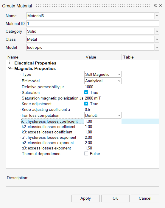 |
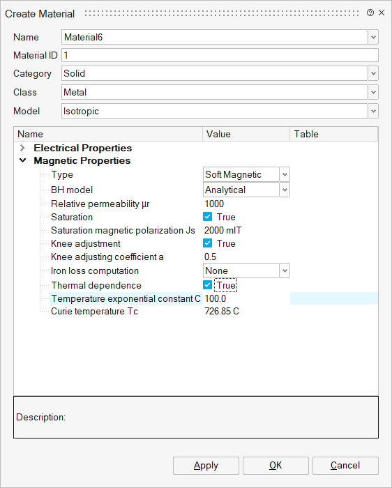
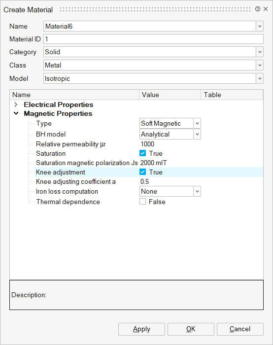
- Open a Create Material dialog box in menu
- Choose Solid as Category field
- Choose Metal as Class field
- In Magnetic Properties:
- Choose Soft Magnetic type
- Choose Analytical BH model
- Define Relative permeability
- Activate Saturation and define Saturation magnetic polarisation Js
- Activate Knee adjustment and define Knee adjustment coefficient a
- In Iron loss computation
- choose None to don't take into
account Iron Loss computation
or
- Choose Bertotti and define coefficients and exponents of Bertotti Model
Note: More details about Iron Losses and Bertotti Model - choose None to don't take into
account Iron Loss computation
- Activate Thermal dependence and define
corresponding parameters (optional)
- Define Temperature exponential constant C
- Define Curie temperature Tc