/FAIL/ORTHBIQUAD

Block Format Keyword This failure model uses an orthotropic simplified nonlinear, plastic strain-based, failure criteria with linear damage accumulation.

For several loading directions, the failure strain is described by two parabolic functions calculated using curve fitting from up to 5 user input failure strains. For all loading directions that are not given in the input, an interpolation of the failure strain evolution with stress triaxiality will be done during the simulation. You can give up to 10 different set of parameters for 10 different directions equally distributed between 1st material direction (0 degree) and 2nd material direction (90 degrees).

Format

(1) (2) (3) (4) (5) (6) (7) (8) (9) (10)
/FAIL/ORTHBIQUAD/mat_ID/unit_ID
Card 1 - Damage accumulation parameters
(1) (2) (3) (4) (5) (6) (7) (8) (9) (10)
P_thickfail M-Flag S-Flag Nangle   fct_IDel El_ref
Card 2 – Biaxial tension failure strain and strain rate dependency
(1) (2) (3) (4) (5) (6) (7) (8) (9) (10)
c5 ε ˙ 0 CJC fct_IDrate Rate_Scale
Optional line (if M_Flag = 99)
(1) (2) (3) (4) (5) (6) (7) (8) (9) (10)
r1 r2 r4 r5
Card 3 - Read Nangle (Number of experimental angles, at least 1) cards
(1) (2) (3) (4) (5) (6) (7) (8) (9) (10)
c1 c2 c3 c4 Inst_start
Optional line
(1) (2) (3) (4) (5) (6) (7) (8) (9) (10)
fail_ID

Definition

Field Contents SI Unit Example
mat_ID Material identifier.

(Integer, maximum 10 digits)

unit_ID (Optional) Unit Identifier.

(Integer, maximum 10 digits)

P_thickfail Ratio of through thickness integration points that must fail before the element is deleted. (shells only).

Default = 1.0 (Real)

M-Flag Material selector flag.
= 0 (Default)
Enter c1 – c5 values
= 1
Mild steel
= 2
HSS steel
= 3
UHSS steel
= 4
Aluminum AA5182
= 5
Aluminum AA6082-T6
= 6
Plastic PA6GF30
= 7
Plastic PP T40
= 99
Enter user-defined failure strain ratios, r1, r2, r4, and r5.

(Integer)

S-Flag Specific behavior flag.
= 1
Two quadratic functions are used.
= 2 (Default)
Plane strain is global minimum.
= 3
Plane strain is global minimum + localized necking.
Nangle Number of experimental angles.

(Integer)

fct_IDel Element size factor function identifier.

(Integer)

El_ref Reference element size.

Default = 1.0 (Real)

[ m ]
c5 Failure plastic strain in biaxial tension (same for all directions).

Default = 0.0 (Real)

ε ˙ 0 Inviscid limit for the strain rate.

Default = 0.0 (Real)

[ 1 s ]
CJC Johnson-Cook strain rate coefficient.

Default = 0.0 (Real)

fct_IDrate Strain rate dependency factor tabulated function identifier.

(Integer)

Rate_Scale Abscissa scale factor for strain rate dependency tabulated function.

Default = 1.0 (Real)

[ 1 s ]
r1 Failure plastic strain ratio, uniaxial compression (c1) to uniaxial tension (c3), so c1=r1c3 MathType@MTEF@5@5@+= feaagKart1ev2aqatCvAUfeBSjuyZL2yd9gzLbvyNv2CaerbuLwBLn hiov2DGi1BTfMBaeXatLxBI9gBaerbd9wDYLwzYbItLDharqqtubsr 4rNCHbGeaGqiVu0Je9sqqrpepC0xbbL8F4rqqrFfpeea0xe9Lq=Jc9 vqaqpepm0xbba9pwe9Q8fs0=yqaqpepae9pg0FirpepeKkFr0xfr=x fr=xb9adbaqaaeGaciGaaiaabeqaamaabaabaaGcbaGaam4yaiaaig dacqGH9aqpcaWGYbGaaGymaiabgwSixlaadogacaaIZaaaaa@3E41@ .

Only used if M-Flag = 99.

Default = 0.0 (Real)

r2 Failure plastic strain ratio, pure shear (c2) to uniaxial tension (c3), so c 2 = r 2 c 3 MathType@MTEF@5@5@+= feaagKart1ev2aqatCvAUfeBSjuyZL2yd9gzLbvyNv2CaerbuLwBLn hiov2DGi1BTfMBaeXatLxBI9gBaerbd9wDYLwzYbItLDharqqtubsr 4rNCHbGeaGqiVu0Je9sqqrpepC0xbbL8F4rqqrFfpeea0xe9Lq=Jc9 vqaqpepm0xbba9pwe9Q8fs0=yqaqpepae9pg0FirpepeKkFr0xfr=x fr=xb9adbaqaaeGaciGaaiaabeqaamaabaabaaGcbaGaam4yaiaaig dacqGH9aqpcaWGYbGaaGymaiabgwSixlaadogacaaIZaaaaa@3E41@ .

Only used if M-Flag = 99.

Default = 0.0 (Real)

r4 Failure plastic strain ratio, plane strain tension (c4) to uniaxial tension (c3), so c 4 = r 4 c 3 MathType@MTEF@5@5@+= feaagKart1ev2aqatCvAUfeBSjuyZL2yd9gzLbvyNv2CaerbuLwBLn hiov2DGi1BTfMBaeXatLxBI9gBaerbd9wDYLwzYbItLDharqqtubsr 4rNCHbGeaGqiVu0Je9sqqrpepC0xbbL8F4rqqrFfpeea0xe9Lq=Jc9 vqaqpepm0xbba9pwe9Q8fs0=yqaqpepae9pg0FirpepeKkFr0xfr=x fr=xb9adbaqaaeGaciGaaiaabeqaamaabaabaaGcbaGaam4yaiaaig dacqGH9aqpcaWGYbGaaGymaiabgwSixlaadogacaaIZaaaaa@3E41@ .

Only used if M-Flag = 99.

Default = 0.0 (Real)

r5 Failure plastic strain ratio, biaxial tension (c5) to uniaxial tension (c3), so c 5 = r 5 c 3 MathType@MTEF@5@5@+= feaagKart1ev2aqatCvAUfeBSjuyZL2yd9gzLbvyNv2CaerbuLwBLn hiov2DGi1BTfMBaeXatLxBI9gBaerbd9wDYLwzYbItLDharqqtubsr 4rNCHbGeaGqiVu0Je9sqqrpepC0xbbL8F4rqqrFfpeea0xe9Lq=Jc9 vqaqpepm0xbba9pwe9Q8fs0=yqaqpepae9pg0FirpepeKkFr0xfr=x fr=xb9adbaqaaeGaciGaaiaabeqaamaabaabaaGcbaGaam4yaiaaig dacqGH9aqpcaWGYbGaaGymaiabgwSixlaadogacaaIZaaaaa@3E41@ .

Only used if M-Flag = 99.

Default = 0.0 (Real)

c1 Failure plastic strain in uniaxial compression.

Default = 0.0 (Real)

c2 Failure plastic strain in shear.

Default = 0.0 (Real)

c3 Failure plastic strain in uniaxial tension.

Default = 0.0 (Real)

c4 Failure plastic strain in plane strain tension.

Default = 0.0 (Real)

Inst_start Instability start value for localized necking.

Must be entered, if S-Flag = 3.

(Real)

fail_ID (Optional) Failure criteria identifier.

(Integer, maximum 10 digits)

Example 1

M-Flag0; M-Flag99: use roughly pre-defined material data (only recommended for early design exploration)
#RADIOSS STARTER
#---1----|----2----|----3----|----4----|----5----|----6----|----7----|----8----|----9----|---10----|
/UNIT/1
unit for mat
#              MUNIT               LUNIT               TUNIT
                  Mg                  mm                   s
#---1----|----2----|----3----|----4----|----5----|----6----|----7----|----8----|----9----|---10----|
#-  1. MATERIALS:
#---1----|----2----|----3----|----4----|----5----|----6----|----7----|----8----|----9----|---10----|
/MAT/LAW93/2/1
Steel
#              RHO_I
             7.8E-09
#                E11                 E22                 E33                 G12                Nu12
              190000              190000              190000               70000                 0.3
#                G13                 G23                Nu13                Nu23
               70000               70000                 0.3                 0.3
#       NL        VP                Fcut
         0         1                   0
#               SigY                 QR1                 CR1                 QR2                 CR2
                 290                 580                   1                 200                  25
#                R11                 R22                 R12
                   1                   1                   1
#                R33                 R13                 R23
                   1                   1                   1
#---1----|----2----|----3----|----4----|----5----|----6----|----7----|----8----|----9----|---10----|
/FAIL/ORTHBIQUAD/2/1
#               PTHK     MFLAG     SFLAG    NANGLE                      FCT_IDEL              EL_REF
                   1         2         1         2                           101                  .3
#                 C5               DEPS0             C_JCOOK         FCT_ID_RATE          RATE_SCALE
                   0                   0                   0                   0                   0
#                 C1                  C2                  C3                  C4                INST
                   0                   0                  .7                   0                  .3
                   0                   0                 .35                   0                 .15
#---1----|----2----|----3----|----4----|----5----|----6----|----7----|----8----|----9----|---10----|
/FUNCT/101
Regularization DP450_ODG3_MED-5
                   0                   1
                   1                   1
                   6                 .35
                  10                 .35
#---1----|----2----|----3----|----4----|----5----|----6----|----7----|----8----|----9----|---10----|
#enddata
#---1----|----2----|----3----|----4----|----5----|----6----|----7----|----8----|----9----|---10----|

Example 2

With M-Flag = 0 and S-flag = 3: input failure strain in c1c5 values
#RADIOSS STARTER
#---1----|----2----|----3----|----4----|----5----|----6----|----7----|----8----|----9----|---10----|
/UNIT/1
unit for mat
#              MUNIT               LUNIT               TUNIT
                  Mg                  mm                   s
#---1----|----2----|----3----|----4----|----5----|----6----|----7----|----8----|----9----|---10----|
#-  1. MATERIALS:
#---1----|----2----|----3----|----4----|----5----|----6----|----7----|----8----|----9----|---10----|
/MAT/LAW93/2/1
Steel
#              RHO_I
             7.8E-09
#                E11                 E22                 E33                 G12                Nu12
              190000              190000              190000               70000                 0.3
#                G13                 G23                Nu13                Nu23
               70000               70000                 0.3                 0.3
#       NL        VP                Fcut
         0         1                   0
#               SigY                 QR1                 CR1                 QR2                 CR2
                 290                 580                   1                 200                  25
#                R11                 R22                 R12
                   1                   1                   1
#                R33                 R13                 R23
                   1                   1                   1
#---1----|----2----|----3----|----4----|----5----|----6----|----7----|----8----|----9----|---10----|
/FAIL/ORTHBIQUAD/2/1
#               PTHK     MFLAG     SFLAG    NANGLE                      FCT_IDEL              EL_REF
                   1         0         1         2                           101                  .3
#                 C5               DEPS0             C_JCOOK         FCT_ID_RATE          RATE_SCALE
                 .56                   0                   0                   0                   0
#                 C1                  C2                  C3                  C4                INST
                3.01                 .98                  .7                 .42                  .3
               1.505                 .49                 .35                 .21                 .15
#---1----|----2----|----3----|----4----|----5----|----6----|----7----|----8----|----9----|---10----|
/FUNCT/101
Regularization DP450_ODG3_MED-5
                   0                   1
                   1                   1
                   6                 .35
                  10                 .35
#---1----|----2----|----3----|----4----|----5----|----6----|----7----|----8----|----9----|---10----|
#enddata
#---1----|----2----|----3----|----4----|----5----|----6----|----7----|----8----|----9----|---10----|

Example 3

With M-Flag = 99 and Johnson-Cook strain rate dependency: input failure strain in c3 and scale of failure strain r1, r2, r4, r5
#RADIOSS STARTER
#---1----|----2----|----3----|----4----|----5----|----6----|----7----|----8----|----9----|---10----|
/UNIT/1
unit for mat
#              MUNIT               LUNIT               TUNIT
                  Mg                  mm                   s
#---1----|----2----|----3----|----4----|----5----|----6----|----7----|----8----|----9----|---10----|
#-  1. MATERIALS:
#---1----|----2----|----3----|----4----|----5----|----6----|----7----|----8----|----9----|---10----|
/MAT/LAW93/2/1
Steel
#              RHO_I
             7.8E-09
#                E11                 E22                 E33                 G12                Nu12
              190000              190000              190000               70000                 0.3
#                G13                 G23                Nu13                Nu23
               70000               70000                 0.3                 0.3
#       NL        VP                Fcut
         0         1                   0
#               SigY                 QR1                 CR1                 QR2                 CR2
                 290                 580                   1                 200                  25
#                R11                 R22                 R12
                   1                   1                   1
#                R33                 R13                 R23
                   1                   1                   1
#---1----|----2----|----3----|----4----|----5----|----6----|----7----|----8----|----9----|---10----|
/FAIL/ORTHBIQUAD/2/1
#               PTHK     MFLAG     SFLAG    NANGLE                      FCT_IDEL              EL_REF
                   1        99         1         2                           101                  .3
#                 C5               DEPS0             C_JCOOK         FCT_ID_RATE          RATE_SCALE
                   0                   0                   0                   0                   0
#                 r1                  r2                  r4                  r5
                 4.3                 1.4                  .6                 1.6
#                 C1                  C2                  C3                  C4                INST
                   0                   0                  .7                   0                  .3
                   0                   0                 .35                   0                 .15
#---1----|----2----|----3----|----4----|----5----|----6----|----7----|----8----|----9----|---10----|
/FUNCT/101
Regularization DP450_ODG3_MED-5
                   0                   1
                   1                   1
                   6                 .35
                  10                 .35
#---1----|----2----|----3----|----4----|----5----|----6----|----7----|----8----|----9----|---10----|
#enddata
#---1----|----2----|----3----|----4----|----5----|----6----|----7----|----8----|----9----|---10----|

Comments

  1. For each input direction, the failure criteria is defined using failure plastic strain versus stress triaxiality (state of stress) as it is the case for the /FAIL/BIQUAD criterion. This allows for the different plastic failure strains that materials exhibit depending on loading condition. The curve is described by 2 parabolic functions that intersect at the triaxiality value of 1 3 MathType@MTEF@5@5@+= feaagKart1ev2aaatCvAUfeBSjuyZL2yd9gzLbvyNv2CaerbuLwBLn hiov2DGi1BTfMBaeXatLxBI9gBaerbd9wDYLwzYbItLDharqqtubsr 4rNCHbGeaGqiVu0Je9sqqrpepC0xbbL8F4rqqrFfpeea0xe9Lq=Jc9 vqaqpepm0xbba9pwe9Q8fs0=yqaqpepae9pg0FirpepeKkFr0xfr=x fr=xb9adbaqaaeGaciGaaiaabeqaamaabaabaaGcbaWaaSaaaeaaca aIXaaabaGaaG4maaaaaaa@377E@ which is uniaxial tension.


    Figure 1. Biquad failure criterion shape

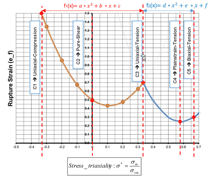
    The parameters for the 2 parabolic failure strain curves versus the state of stress (stress triaxiality) are calculated iteratively by Radioss during the initialization phase using the input c1-c5 values.

    If the calculated parabolic failure strain curves have negative failure strain values, these negative values will be replaced by a failure strain of 1E-6 which results in a very high damage accumulation and brittle behavior.

    This failure criteria is usable for all elasto-plastic material models with shells and solids.

  2. To consider the failure orthotropy, several set of c1, c2, c3, c4 and Inst_start parameters can be given. You can input up to 10 different set of parameters for 10 different experimental loading directions (marked by an angle denoted θ ). The number of input tested loading direction is set by the parameter Nangle. The directions must be equally distributed, 1st material direction (0 degree) and 2nd material direction (90 degrees) following the table. For isotropic material laws, the elemental system is used: directions are distributed between the local element x-axis (0 degree) and local element y-axis (90 degrees).


    Figure 2. Expected input loading direction angle depending on the value of Nangle
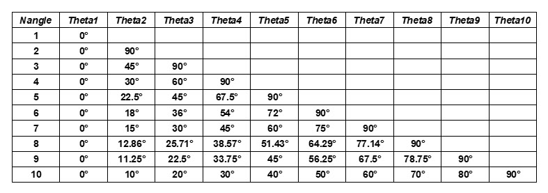
  3. For each input direction, the 2 parabolic curves parameters ( a MathType@MTEF@5@5@+= feaagKart1ev2aaatCvAUfeBSjuyZL2yd9gzLbvyNv2CaerbuLwBLn hiov2DGi1BTfMBaeXatLxBI9gBaerbd9wDYLwzYbItLDharqqtubsr 4rNCHbGeaGqipu0Je9sqqrpepC0xbbL8F4rqqrFfpeea0xe9Lq=Jc9 vqaqpepm0xbba9pwe9Q8fs0=yqaqpepae9pg0FirpepeKkFr0xfr=x fr=xb9adbaqaaeGaciGaaiaabeqaamaabaabaaGcbaGaamyyaaaa@36BC@ , b MathType@MTEF@5@5@+= feaagKart1ev2aaatCvAUfeBSjuyZL2yd9gzLbvyNv2CaerbuLwBLn hiov2DGi1BTfMBaeXatLxBI9gBaerbd9wDYLwzYbItLDharqqtubsr 4rNCHbGeaGqipu0Je9sqqrpepC0xbbL8F4rqqrFfpeea0xe9Lq=Jc9 vqaqpepm0xbba9pwe9Q8fs0=yqaqpepae9pg0FirpepeKkFr0xfr=x fr=xb9adbaqaaeGaciGaaiaabeqaamaabaabaaGcbaGaamyyaaaa@36BC@ , c MathType@MTEF@5@5@+= feaagKart1ev2aaatCvAUfeBSjuyZL2yd9gzLbvyNv2CaerbuLwBLn hiov2DGi1BTfMBaeXatLxBI9gBaerbd9wDYLwzYbItLDharqqtubsr 4rNCHbGeaGqipu0Je9sqqrpepC0xbbL8F4rqqrFfpeea0xe9Lq=Jc9 vqaqpepm0xbba9pwe9Q8fs0=yqaqpepae9pg0FirpepeKkFr0xfr=x fr=xb9adbaqaaeGaciGaaiaabeqaamaabaabaaGcbaGaamyyaaaa@36BC@ , d MathType@MTEF@5@5@+= feaagKart1ev2aaatCvAUfeBSjuyZL2yd9gzLbvyNv2CaerbuLwBLn hiov2DGi1BTfMBaeXatLxBI9gBaerbd9wDYLwzYbItLDharqqtubsr 4rNCHbGeaGqipu0Je9sqqrpepC0xbbL8F4rqqrFfpeea0xe9Lq=Jc9 vqaqpepm0xbba9pwe9Q8fs0=yqaqpepae9pg0FirpepeKkFr0xfr=x fr=xb9adbaqaaeGaciGaaiaabeqaamaabaabaaGcbaGaamyyaaaa@36BC@ , e MathType@MTEF@5@5@+= feaagKart1ev2aaatCvAUfeBSjuyZL2yd9gzLbvyNv2CaerbuLwBLn hiov2DGi1BTfMBaeXatLxBI9gBaerbd9wDYLwzYbItLDharqqtubsr 4rNCHbGeaGqipu0Je9sqqrpepC0xbbL8F4rqqrFfpeea0xe9Lq=Jc9 vqaqpepm0xbba9pwe9Q8fs0=yqaqpepae9pg0FirpepeKkFr0xfr=x fr=xb9adbaqaaeGaciGaaiaabeqaamaabaabaaGcbaGaamyyaaaa@36BC@ , f MathType@MTEF@5@5@+= feaagKart1ev2aaatCvAUfeBSjuyZL2yd9gzLbvyNv2CaerbuLwBLn hiov2DGi1BTfMBaeXatLxBI9gBaerbd9wDYLwzYbItLDharqqtubsr 4rNCHbGeaGqipu0Je9sqqrpepC0xbbL8F4rqqrFfpeea0xe9Lq=Jc9 vqaqpepm0xbba9pwe9Q8fs0=yqaqpepae9pg0FirpepeKkFr0xfr=x fr=xb9adbaqaaeGaciGaaiaabeqaamaabaabaaGcbaGaamyyaaaa@36BC@ ) are computed in the Radioss Starter. During the simulation, for all loading directions located between the input directions, a Fourier series interpolation is used to determine the corresponding curves parameters ( a MathType@MTEF@5@5@+= feaagKart1ev2aaatCvAUfeBSjuyZL2yd9gzLbvyNv2CaerbuLwBLn hiov2DGi1BTfMBaeXatLxBI9gBaerbd9wDYLwzYbItLDharqqtubsr 4rNCHbGeaGqipu0Je9sqqrpepC0xbbL8F4rqqrFfpeea0xe9Lq=Jc9 vqaqpepm0xbba9pwe9Q8fs0=yqaqpepae9pg0FirpepeKkFr0xfr=x fr=xb9adbaqaaeGaciGaaiaabeqaamaabaabaaGcbaGaamyyaaaa@36BC@ , b MathType@MTEF@5@5@+= feaagKart1ev2aaatCvAUfeBSjuyZL2yd9gzLbvyNv2CaerbuLwBLn hiov2DGi1BTfMBaeXatLxBI9gBaerbd9wDYLwzYbItLDharqqtubsr 4rNCHbGeaGqipu0Je9sqqrpepC0xbbL8F4rqqrFfpeea0xe9Lq=Jc9 vqaqpepm0xbba9pwe9Q8fs0=yqaqpepae9pg0FirpepeKkFr0xfr=x fr=xb9adbaqaaeGaciGaaiaabeqaamaabaabaaGcbaGaamyyaaaa@36BC@ , c MathType@MTEF@5@5@+= feaagKart1ev2aaatCvAUfeBSjuyZL2yd9gzLbvyNv2CaerbuLwBLn hiov2DGi1BTfMBaeXatLxBI9gBaerbd9wDYLwzYbItLDharqqtubsr 4rNCHbGeaGqipu0Je9sqqrpepC0xbbL8F4rqqrFfpeea0xe9Lq=Jc9 vqaqpepm0xbba9pwe9Q8fs0=yqaqpepae9pg0FirpepeKkFr0xfr=x fr=xb9adbaqaaeGaciGaaiaabeqaamaabaabaaGcbaGaamyyaaaa@36BC@ , d MathType@MTEF@5@5@+= feaagKart1ev2aaatCvAUfeBSjuyZL2yd9gzLbvyNv2CaerbuLwBLn hiov2DGi1BTfMBaeXatLxBI9gBaerbd9wDYLwzYbItLDharqqtubsr 4rNCHbGeaGqipu0Je9sqqrpepC0xbbL8F4rqqrFfpeea0xe9Lq=Jc9 vqaqpepm0xbba9pwe9Q8fs0=yqaqpepae9pg0FirpepeKkFr0xfr=x fr=xb9adbaqaaeGaciGaaiaabeqaamaabaabaaGcbaGaamyyaaaa@36BC@ , e MathType@MTEF@5@5@+= feaagKart1ev2aaatCvAUfeBSjuyZL2yd9gzLbvyNv2CaerbuLwBLn hiov2DGi1BTfMBaeXatLxBI9gBaerbd9wDYLwzYbItLDharqqtubsr 4rNCHbGeaGqipu0Je9sqqrpepC0xbbL8F4rqqrFfpeea0xe9Lq=Jc9 vqaqpepm0xbba9pwe9Q8fs0=yqaqpepae9pg0FirpepeKkFr0xfr=x fr=xb9adbaqaaeGaciGaaiaabeqaamaabaabaaGcbaGaamyyaaaa@36BC@ , f MathType@MTEF@5@5@+= feaagKart1ev2aaatCvAUfeBSjuyZL2yd9gzLbvyNv2CaerbuLwBLn hiov2DGi1BTfMBaeXatLxBI9gBaerbd9wDYLwzYbItLDharqqtubsr 4rNCHbGeaGqipu0Je9sqqrpepC0xbbL8F4rqqrFfpeea0xe9Lq=Jc9 vqaqpepm0xbba9pwe9Q8fs0=yqaqpepae9pg0FirpepeKkFr0xfr=x fr=xb9adbaqaaeGaciGaaiaabeqaamaabaabaaGcbaGaamyyaaaa@36BC@ ) and, if defined, the necking instability strain (Inst_start):(1)
    a = m = 0 N a n g l e Q m a cos ( 2 m θ ) d = m = 0 N a n g l e Q m d cos ( 2 m θ ) b = m = 0 N a n g l e Q m b cos ( 2 m θ ) e = m = 0 N a n g l e Q m e cos ( 2 m θ ) I n s t = m = 0 N a n g l e Q m I n s t cos ( 2 m θ ) c = m = 0 N a n g l e Q m c cos ( 2 m θ ) f = m = 0 N a n g l e Q m f cos ( 2 m θ ) MathType@MTEF@5@5@+= feaagKart1ev2aaatCvAUfeBSjuyZL2yd9gzLbvyNv2CaerbuLwBLn hiov2DGi1BTfMBaeXatLxBI9gBaerbd9wDYLwzYbItLDharqqtubsr 4rNCHbGeaGqiVu0Je9sqqrpepC0xbbL8F4rqqrFfpeea0xe9Lq=Jc9 vqaqpepm0xbba9pwe9Q8fs0=yqaqpepae9pg0FirpepeKkFr0xfr=x fr=xb9adbaqaaeGaciGaaiaabeqaamaabaabaaGcbaqbaeqabmWaaa qaaiaadggacqGH9aqpdaaeWbqaaiaadgfadaqhaaWcbaGaamyBaaqa aiaadggaaaGcciGGJbGaai4BaiaacohacaGGOaGaaGOmaiaad2gacq aH4oqCcaGGPaaaleaacaWGTbGaeyypa0JaaGimaaqaaiaad6eadaWg aaadbaGaamyyaiaad6gacaWGNbGaamiBaiaadwgaaeqaaaqdcqGHri s5aaGcbaGaamizaiabg2da9maaqahabaGaamyuamaaDaaaleaacaWG TbaabaGaamizaaaakiGacogacaGGVbGaai4CaiaacIcacaaIYaGaam yBaiabeI7aXjaacMcaaSqaaiaad2gacqGH9aqpcaaIWaaabaGaamOt amaaBaaameaacaWGHbGaamOBaiaadEgacaWGSbGaamyzaaqabaaani abggHiLdaakeaaaeaacaWGIbGaeyypa0ZaaabCaeaacaWGrbWaa0ba aSqaaiaad2gaaeaacaWGIbaaaOGaci4yaiaac+gacaGGZbGaaiikai aaikdacaWGTbGaeqiUdeNaaiykaaWcbaGaamyBaiabg2da9iaaicda aeaacaWGobWaaSbaaWqaaiaadggacaWGUbGaam4zaiaadYgacaWGLb aabeaaa0GaeyyeIuoaaOqaaiaadwgacqGH9aqpdaaeWbqaaiaadgfa daqhaaWcbaGaamyBaaqaaiaadwgaaaGcciGGJbGaai4Baiaacohaca GGOaGaaGOmaiaad2gacqaH4oqCcaGGPaaaleaacaWGTbGaeyypa0Ja aGimaaqaaiaad6eadaWgaaadbaGaamyyaiaad6gacaWGNbGaamiBai aadwgaaeqaaaqdcqGHris5aaGcbaGaamysaiaad6gacaWGZbGaamiD aiabg2da9maaqahabaGaamyuamaaDaaaleaacaWGTbaabaGaamysai aad6gacaWGZbGaamiDaaaakiGacogacaGGVbGaai4CaiaacIcacaaI YaGaamyBaiabeI7aXjaacMcaaSqaaiaad2gacqGH9aqpcaaIWaaaba GaamOtamaaBaaameaacaWGHbGaamOBaiaadEgacaWGSbGaamyzaaqa baaaniabggHiLdaakeaacaWGJbGaeyypa0ZaaabCaeaacaWGrbWaa0 baaSqaaiaad2gaaeaacaWGJbaaaOGaci4yaiaac+gacaGGZbGaaiik aiaaikdacaWGTbGaeqiUdeNaaiykaaWcbaGaamyBaiabg2da9iaaic daaeaacaWGobWaaSbaaWqaaiaadggacaWGUbGaam4zaiaadYgacaWG Lbaabeaaa0GaeyyeIuoaaOqaaiaadAgacqGH9aqpdaaeWbqaaiaadg fadaqhaaWcbaGaamyBaaqaaiaadAgaaaGcciGGJbGaai4Baiaacoha caGGOaGaaGOmaiaad2gacqaH4oqCcaGGPaaaleaacaWGTbGaeyypa0 JaaGimaaqaaiaad6eadaWgaaadbaGaamyyaiaad6gacaWGNbGaamiB aiaadwgaaeqaaaqdcqGHris5aaGcbaaaaaaa@DCBC@

    Where, Q m i MathType@MTEF@5@5@+= feaagKart1ev2aaatCvAUfeBSjuyZL2yd9gzLbvyNv2CaerbuLwBLn hiov2DGi1BTfMBaeXatLxBI9gBaerbd9wDYLwzYbItLDharqqtubsr 4rNCHbGeaGqiVu0Je9sqqrpepC0xbbL8F4rqqrFfpeea0xe9Lq=Jc9 vqaqpepm0xbba9pwe9Q8fs0=yqaqpepae9pg0FirpepeKkFr0xfr=x fr=xb9adbaqaaeGaciGaaiaabeqaamaabaabaaGcbaGaamyuamaaDa aaleaacaWGTbaabaGaamyAaaaaaaa@38D9@ are the interpolation factors for parameter i MathType@MTEF@5@5@+= feaagKart1ev2aaatCvAUfeBSjuyZL2yd9gzLbvyNv2CaerbuLwBLn hiov2DGi1BTfMBaeXatLxBI9gBaerbd9wDYLwzYbItLDharqqtubsr 4rNCHbGeaGqipu0Je9sqqrpepC0xbbL8F4rqqrFfpeea0xe9Lq=Jc9 vqaqpepm0xbba9pwe9Q8fs0=yqaqpepae9pg0FirpepeKkFr0xfr=x fr=xb9adbaqaaeGaciGaaiaabeqaamaabaabaaGcbaGaamyyaaaa@36BC@ . These interpolation factors are automatically computed in the Radioss Starter.

    For instance, if two sets of parameters are given for the direction 0 and 90 degrees, the Fourier series interpolation enables to determine the 45 degrees curve as:


    Figure 3. Example of orthotropic biquad criterion shape

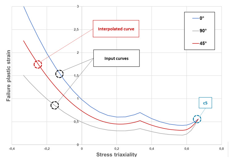
    Loading directions not given in the input are interpolated using Fourier series. All directions have the same plastic strain at failure in biaxial tension.

  4. It must be noted that plastic strain at failure in biaxial tension c5 is common to all directions (Figure 3). Indeed, for this loading condition, the directions have no meaning as all directions are loaded in the same way. Thus, the failure behavior is the same.
  5. By default, values different than 0 for c1 to c5 need to be entered. However, specific default behaviors exist in case failure information are missing:
    • In case the material failure behavior is unknown, c1 to c5 are set to 0.0 and the mild steel behavior (M-Flag=1) is used.
    • If only the tensile failure value is known, c3 is defined (c1=c2=c4=c5 = 0.0). The mild steel behavior is used and scaled by the user-defined c3 value.
    • In case the material behavior is known, M-Flag is defined and c3 can be used to adjust the failure model according to the expected tensile failure. The selected material behavior is scaled by the user-defined c3 value.
    • For all other cases, all c1 to c5 are intended to be defined and default value of 0.0 is used.
      Note: If c5 = 0.0, it is automatically computed depending on the value of M-Flag. In this case, the minimum value computed among all input directions will be retained.
  6. The plastic strain at failure from physical tests can be input as c1c5.
  7. If failure strain data is not available then the material flag, M-Flag, can be used to select predefined failure values for some materials.
    • If M-Flag > 0, the entered c1, c2, c4 and c5 values will not be used, but will be calculated as follows, using the predefined ratio values from the table.

      c 1 = r 1 c 3 MathType@MTEF@5@5@+= feaagKart1ev2aqatCvAUfeBSjuyZL2yd9gzLbvyNv2CaerbuLwBLn hiov2DGi1BTfMBaeXatLxBI9gBaerbd9wDYLwzYbItLDharqqtubsr 4rNCHbGeaGqiVu0Je9sqqrpepC0xbbL8F4rqqrFfpeea0xe9Lq=Jc9 vqaqpepm0xbba9pwe9Q8fs0=yqaqpepae9pg0FirpepeKkFr0xfr=x fr=xb9adbaqaaeGaciGaaiaabeqaamaabaabaaGcbaGaam4yaiaaig dacqGH9aqpcaWGYbGaaGymaiabgwSixlaadogacaaIZaaaaa@3E41@

      c 2 = r 2 c 3 MathType@MTEF@5@5@+= feaagKart1ev2aqatCvAUfeBSjuyZL2yd9gzLbvyNv2CaerbuLwBLn hiov2DGi1BTfMBaeXatLxBI9gBaerbd9wDYLwzYbItLDharqqtubsr 4rNCHbGeaGqiVu0Je9sqqrpepC0xbbL8F4rqqrFfpeea0xe9Lq=Jc9 vqaqpepm0xbba9pwe9Q8fs0=yqaqpepae9pg0FirpepeKkFr0xfr=x fr=xb9adbaqaaeGaciGaaiaabeqaamaabaabaaGcbaGaam4yaiaaik dacqGH9aqpcaWGYbGaaGOmaiabgwSixlaadogacaaIZaaaaa@3E43@

      c 3 = c 3 MathType@MTEF@5@5@+= feaagKart1ev2aqatCvAUfeBSjuyZL2yd9gzLbvyNv2CaerbuLwBLn hiov2DGi1BTfMBaeXatLxBI9gBaerbd9wDYLwzYbItLDharqqtubsr 4rNCHbGeaGqiVu0Je9sqqrpepC0xbbL8F4rqqrFfpeea0xe9Lq=Jc9 vqaqpepm0xbba9pwe9Q8fs0=yqaqpepae9pg0FirpepeKkFr0xfr=x fr=xb9adbaqaaeGaciGaaiaabeqaamaabaabaaGcbaGaam4yaiaaio dacqGH9aqpcaWGJbGaaG4maaaa@3A47@

      c 4 = r 4 c 3 MathType@MTEF@5@5@+= feaagKart1ev2aqatCvAUfeBSjuyZL2yd9gzLbvyNv2CaerbuLwBLn hiov2DGi1BTfMBaeXatLxBI9gBaerbd9wDYLwzYbItLDharqqtubsr 4rNCHbGeaGqiVu0Je9sqqrpepC0xbbL8F4rqqrFfpeea0xe9Lq=Jc9 vqaqpepm0xbba9pwe9Q8fs0=yqaqpepae9pg0FirpepeKkFr0xfr=x fr=xb9adbaqaaeGaciGaaiaabeqaamaabaabaaGcbaGaam4yaiaais dacqGH9aqpcaWGYbGaaGinaiabgwSixlaadogacaaIZaaaaa@3E47@

      c 5 = r 5 c 3 MathType@MTEF@5@5@+= feaagKart1ev2aqatCvAUfeBSjuyZL2yd9gzLbvyNv2CaerbuLwBLn hiov2DGi1BTfMBaeXatLxBI9gBaerbd9wDYLwzYbItLDharqqtubsr 4rNCHbGeaGqiVu0Je9sqqrpepC0xbbL8F4rqqrFfpeea0xe9Lq=Jc9 vqaqpepm0xbba9pwe9Q8fs0=yqaqpepae9pg0FirpepeKkFr0xfr=x fr=xb9adbaqaaeGaciGaaiaabeqaamaabaabaaGcbaGaam4yaiaaiw dacqGH9aqpcaWGYbGaaGynaiabgwSixlaadogacaaIZaaaaa@3E49@

    • If c3=0, the default value shown in the table is used.
      M-Flag Roughly Corresponds to Material c3

      (Default)

      r1 r2 r4 r5
      1 Mild steel 0.60 3.5 1.6 0.6 1.5
      2 HSS steel 0.50 4.3 1.4 0.6 1.6
      3 UHSS steel 0.12 5.2 3.1 0.8 3.5
      4 Aluminum AA5182 0.30 5.0 1.0 0.4 0.8
      5 Aluminum AA6082-T6 0.17 7.8 3.5 0.6 2.8
      6 Plastic PA6GF30 0.10 3.6 0.6 0.5 0.6
      7 Plastic PP T40 0.11 10.0 2.7 0.6 0.7
      99 Self-defined values (optional line) 0.30 Optional input Optional input Optional input Optional input
      Important: Neither Altair nor the authors assume any responsibility for the validity, accuracy or any results obtained from these values. You must verify your own values by reasonable test results. Usage is only recommended for early design exploration.
    • If c3 > 0, the selected material behavior is scaled by c3 and the r1 to r5 predefined ratio values.
    • If c5 = 0.0, the minimum value of among all input directions will be retained.
    • If the M-Flag = 99, failure strain ratios r1, r2, r4 and r5 must be input in a following additional line.
  8. Damage is accumulated linearly and can be post-processed in the animation files using the output request /ANIM/SHELL/DAMA/ALL or /ANIM/BRICK/DAMA/111.(2)
    D = t = 0 Δ ε p ε f θ ( η ) MathType@MTEF@5@5@+= feaagKart1ev2aqatCvAUfeBSjuyZL2yd9gzLbvyNv2CaerbuLwBLn hiov2DGi1BTfMBaeXatLxBI9gBaerbd9wDYLwzYbItLDharqqtubsr 4rNCHbGeaGqiVu0Je9sqqrpepC0xbbL8F4rqqrFfpeea0xe9Lq=Jc9 vqaqpepm0xbba9pwe9Q8fs0=yqaqpepae9pg0FirpepeKkFr0xfr=x fr=xb9adbaqaaeGaciGaaiaabeqaamaabaabaaGcbaGaamiraiabg2 da9maaqahabaWaaSaaaeaacqqHuoarcqaH1oqzdaWgaaWcbaGaamiC aaqabaaakeaacqaH1oqzdaqhaaWcbaGaamOzaaqaaiabeI7aXbaaki aacIcacqaH3oaAcaGGPaaaaaWcbaGaamiDaiabg2da9iaaicdaaeaa cqGHEisPa0GaeyyeIuoaaaa@49FE@

    For shell elements when an integration point reaches D = 1 MathType@MTEF@5@5@+= feaagKart1ev2aaatCvAUfeBSjuyZL2yd9gzLbvyNv2CaerbuLwBLn hiov2DGi1BTfMBaeXatLxBI9gBaerbd9wDYLwzYbItLDharqqtubsr 4rNCHbGeaGqiVu0Je9sqqrpepC0xbbL8F4rqqrFfpeea0xe9Lq=Jc9 vqaqpepm0xbbG8FasPYRqj0=yi0dXdbba9pGe9xq=JbbG8A8frFve9 Fve9Ff0dmeaabaqaciGacaGaaeqabaWaaeaaeaaakeaacaWGebGaey ypa0JaaGymaaaa@38E8@ , the integration points stress tensor is set to 0. Shell elements are deleted based on the value of P_thickfail.

    If P_thickfail is set blank or 0, the value of P_thickfail from the shell property is used. If P_thickfail > 0, any P_thickfail value defined in the shell properties is ignored and the value entered in this failure model is used.

    For values of P_thickfail set > 0, the element fails and is deleted when the ratio of through thickness failed integration points equals or exceeds P_thickfail.

    In solid elements, the element is deleted when any integration point reaches D = 1 MathType@MTEF@5@5@+= feaagKart1ev2aaatCvAUfeBSjuyZL2yd9gzLbvyNv2CaerbuLwBLn hiov2DGi1BTfMBaeXatLxBI9gBaerbd9wDYLwzYbItLDharqqtubsr 4rNCHbGeaGqiVu0Je9sqqrpepC0xbbL8F4rqqrFfpeea0xe9Lq=Jc9 vqaqpepm0xbbG8FasPYRqj0=yi0dXdbba9pGe9xq=JbbG8A8frFve9 Fve9Ff0dmeaabaqaciGacaGaaeqabaWaaeaaeaaakeaacaWGebGaey ypa0JaaGymaaaa@38E8@ .

  9. Special features are activated by this flag:
    • S-Flag = 1: the failure curves are created, as shown in Comment 1. In this case, the curves may not reach their minimum value for the same stress triaxiality (Figure 4).


      Figure 4. Orthotropic biquadratic failure criterion shape when S-Flag =1
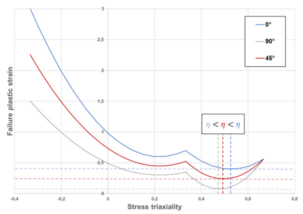
    • S-Flag = 2: is set by default. It ensures value c4 as global minimum for all directions. To achieve this for all curves, the second equation is split into 2 separate quadratic sub-functions where the minimum value of the curves is at c4; where, σ * = 1 3 MathType@MTEF@5@5@+= feaagKart1ev2aqatCvAUfeBSjuyZL2yd9gzLbvyNv2CaerbuLwBLn hiov2DGi1BTfMBaeXatLxBI9gBaerbd9wDYLwzYbItLDharqqtubsr 4rNCHbGeaGqiVu0Je9sqqrpepC0xbbL8F4rqqrFfpeea0xe9Lq=Jc9 vqaqpepm0xbba9pwe9Q8fs0=yqaqpepae9pg0FirpepeKkFr0xfr=x fr=xb9adbaqaaeGaciGaaiaabeqaamaabaabaaGcbaGaeq4Wdm3aaW baaSqabeaacaGGQaaaaOGaeyypa0ZaaSaaaeaacaaIXaaabaWaaOaa aeaacaaIZaaaleqaaaaaaaa@3B48@ (Figure 5).


      Figure 5. Orthotropic biquadratic failure criterion shape when S-Flag =2
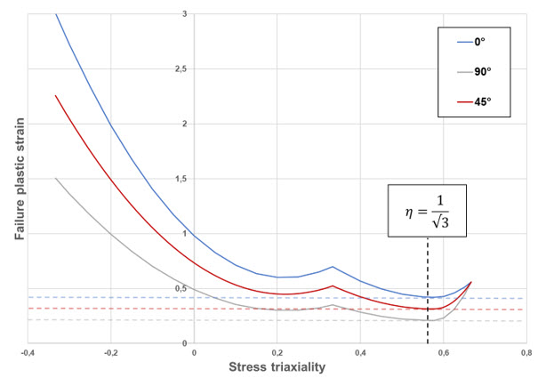
    • S-Flag = 3: same as S-Flag = 2, plus a simplified localized necking criterion (only for shells). The localized necking criteria is based on the Marciniak-Kuczynski analysis. It uses two additional quadratic functions that define a curve that represents the start of localized necking between stress triaxiality 1 3 MathType@MTEF@5@5@+= feaagKart1ev2aaatCvAUfeBSjuyZL2yd9gzLbvyNv2CaerbuLwBLn hiov2DGi1BTfMBaeXatLxBI9gBaerbd9wDYLwzYbItLDharqqtubsr 4rNCHbGeaGqiVCI8FfYJH8YrFfeuY=Hhbbf9v8qqaqFr0xc9pk0xbb a9q8WqFfeaY=biLkVcLq=JHqpepeea0=as0Fb9pgeaYRXxe9vr0=vr 0=vqpWqaaeaabiGaciaacaqabeaadaqaaqaaaOqaamaalaaabaGaaG ymaaqaaiaaiodaaaaaaa@3773@ and 2 3 MathType@MTEF@5@5@+= feaagKart1ev2aaatCvAUfeBSjuyZL2yd9gzLbvyNv2CaerbuLwBLn hiov2DGi1BTfMBaeXatLxBI9gBaerbd9wDYLwzYbItLDharqqtubsr 4rNCHbGeaGqiVCI8FfYJH8YrFfeuY=Hhbbf9v8qqaqFr0xc9pk0xbb a9q8WqFfeaY=biLkVcLq=JHqpepeea0=as0Fb9pgeaYRXxe9vr0=vr 0=vqpWqaaeaabiGaciaacaqabeaadaqaaqaaaOqaamaalaaabaGaaG ymaaqaaiaaiodaaaaaaa@3773@ . The minimum value of this curve is user-defined in the Inst_start field and occurs at plane strain tension, σ * = 1 3 MathType@MTEF@5@5@+= feaagKart1ev2aqatCvAUfeBSjuyZL2yd9gzLbvyNv2CaerbuLwBLn hiov2DGi1BTfMBaeXatLxBI9gBaerbd9wDYLwzYbItLDharqqtubsr 4rNCHbGeaGqiVu0Je9sqqrpepC0xbbL8F4rqqrFfpeea0xe9Lq=Jc9 vqaqpepm0xbbG8FasPYRqj0=yi0dXdbba9pGe9xq=JbbG8A8frFve9 Fve9Ff0dmeaabaqaciGacaGaaeqabaWaaeaaeaaakeaaqaaaaaaaaa Wdbiabeo8aZ9aadaahaaWcbeqaa8qacaGGQaaaaOWdaiabg2da9maa laaabaGaaGymaaqaamaakaaabaGaaG4maaWcbeaaaaaaaa@3BFE@ (Figure 6).

      Using this curve, a second localized necking damage value is calculated, and failure only occurs when all integration points reach D = 1 MathType@MTEF@5@5@+= feaagKart1ev2aaatCvAUfeBSjuyZL2yd9gzLbvyNv2CaerbuLwBLn hiov2DGi1BTfMBaeXatLxBI9gBaerbd9wDYLwzYbItLDharqqtubsr 4rNCHbGeaGqiVu0Je9sqqrpepC0xbbL8F4rqqrFfpeea0xe9Lq=Jc9 vqaqpepm0xbbG8FasPYRqj0=yi0dXdbba9pGe9xq=JbbG8A8frFve9 Fve9Ff0dmeaabaqaciGacaGaaeqabaWaaeaaeaaakeaacaWGebGaey ypa0JaaGymaaaa@38E8@ .

      The Inst_start value can be estimated as the (true plastic) strain at maximum stress, from the uniaxial tension test.


      Figure 6. Orthotropic biquadratic failure criterion shape when S-Flag =3
  10. A strain rate dependency can be applied on the failure criterion, if:
    • ε ˙ 0 0 MathType@MTEF@5@5@+= feaagKart1ev2aqatCvAUfeBSjuyZL2yd9gzLbvyNv2CaerbuLwBLn hiov2DGi1BTfMBaeXatLxBI9gBaerbd9wDYLwzYbItLDharqqtubsr 4rNCHbGeaGqiVu0Je9sqqrpepC0xbbL8F4rqqrFfpeea0xe9Lq=Jc9 vqaqpepm0xbba9pwe9Q8fs0=yqaqpepae9pg0FirpepeKkFr0xfr=x fr=xb9adbaqaaeGaciGaaiaabeqaamaabaabaaGcbaGafqyTduMbai aadaWgaaWcbaGaaGimaaqabaGccqGHGjsUcaaIWaaaaa@3B18@ and C J C 0 MathType@MTEF@5@5@+= feaagKart1ev2aqatCvAUfeBSjuyZL2yd9gzLbvyNv2CaerbuLwBLn hiov2DGi1BTfMBaeXatLxBI9gBaerbd9wDYLwzYbItLDharqqtubsr 4rNCHbGeaGqiVu0Je9sqqrpepC0xbbL8F4rqqrFfpeea0xe9Lq=Jc9 vqaqpepm0xbba9pwe9Q8fs0=yqaqpepae9pg0FirpepeKkFr0xfr=x fr=xb9adbaqaaeGaciGaaiaabeqaamaabaabaaGcbaGaam4qamaaBa aaleaacaWGkbGaam4qaaqabaGccqGHGjsUcaaIWaaaaa@3B0D@ , the Johnson-Cook’s strain rate dependency is used. In this case, the plastic strain at failure value is multiplied by the strain rate dependency factor as:(3)
      D= t=0 Δ ε p ε f θ (η) 1+ C JC ln ε ˙ ε ˙ 0 + MathType@MTEF@5@5@+= feaahqart1ev3aqatCvAUfeBSjuyZL2yd9gzLbvyNv2CaerbuLwBLn hiov2DGi1BTfMBaeXatLxBI9gBaerbd9wDYLwzYbItLDharqqtubsr 4rNCHbGeaGqiVu0Je9sqqrpepC0xbbL8F4rqqrFfpeea0xe9Lq=Jc9 vqaqpepm0xbba9pwe9Q8fs0=yqaqpepae9pg0FirpepeKkFr0xfr=x fr=xb9adbaqaaeGaciGaaiaabeqaamaabaabaaGcbaGaamiraiabg2 da9maaqahabaWaaSaaaeaacqqHuoarcqaH1oqzdaWgaaWcbaGaamiC aaqabaaakeaacqaH1oqzdaqhaaWcbaGaamOzaaqaaiabeI7aXbaaki aacIcacqaH3oaAcaGGPaWaaeWaaeaacaaIXaGaey4kaSIaam4qamaa BaaaleaacaWGkbGaam4qaaqabaGcdaaadaqaaiGacYgacaGGUbWaaS aaaeaacuaH1oqzgaGaaaqaaiqbew7aLzaacaWaaSbaaSqaaiaaicda aeqaaaaaaOGaayzkJiaawQYiamaaBaaaleaacqGHRaWkaeqaaaGcca GLOaGaayzkaaaaaaWcbaGaamiDaiabg2da9iaaicdaaeaacqGHEisP a0GaeyyeIuoaaaa@58E2@
      Where,
      ε ˙ 0
      Inviscid limit strain rate
      C J C MathType@MTEF@5@5@+= feaagKart1ev2aqatCvAUfeBSjuyZL2yd9gzLbvyNv2CaerbuLwBLn hiov2DGi1BTfMBaeXatLxBI9gBaerbd9wDYLwzYbItLDharqqtubsr 4rNCHbGeaGqiVu0Je9sqqrpepC0xbbL8F4rqqrFfpeea0xe9Lq=Jc9 vqaqpepm0xbba9pwe9Q8fs0=yqaqpepae9pg0FirpepeKkFr0xfr=x fr=xb9adbaqaaeGaciGaaiaabeqaamaabaabaaGcbaGaam4qamaaBa aaleaacaWGkbGaam4qaaqabaaaaa@3882@
      Strain rate dependency parameter
      + MathType@MTEF@5@5@+= feaagKart1ev2aaatCvAUfeBSjuyZL2yd9gzLbvyNv2CaerbuLwBLn hiov2DGi1BTfMBaeXatLxBI9gBaerbd9wDYLwzYbItLDharqqtubsr 4rNCHbGeaGqiVu0Je9sqqrpepC0xbbL8F4rqqrFfpeea0xe9Lq=Jc9 vqaqpepm0xbba9pwe9Q8fs0=yqaqpepae9pg0FirpepeKkFr0xfr=x fr=xb9adbaqaaeGaciGaaiaabeqaamaabaabaaGcbaWaaaWaaeaaai aawMYicaGLQmcadaWgaaWcbaGaey4kaScabeaaaaa@38D4@
      Macaulay brackets, which considers only positive values
      Note: If using a Johnson-Cook material law coupled to the /FAIL/ORTHBIQUAD criterion, the Johnson-Cook parameters used for the constitutive law might not be the same for the failure criterion.
    • fct_IDrate ≠ 0, a tabulated function of strain rate dependency factor is used. In this case, you have to define a function (/FUNCT) to describe the evolution of the strain rate factor (denoted f r a t e MathType@MTEF@5@5@+= feaagKart1ev2aqatCvAUfeBSjuyZL2yd9gzLbvyNv2CaerbuLwBLn hiov2DGi1BTfMBaeXatLxBI9gBaerbd9wDYLwzYbItLDharqqtubsr 4rNCHbGeaGqiVu0Je9sqqrpepC0xbbL8F4rqqrFfpeea0xe9Lq=Jc9 vqaqpepm0xbba9pwe9Q8fs0=yqaqpepae9pg0FirpepeKkFr0xfr=x fr=xb9adbaqaaeGaciGaaiaabeqaamaabaabaaGcbaGaamOzamaaBa aaleaacaWGYbGaamyyaiaadshacaWGLbaabeaaaaa@3ACE@ ) with the strain rate. You can also input a strain rate scale factor for the abscissa of the function: Xscale_rate (by default, this scale factor is set to 1.0). Using the tabulated strain rate dependency, the damage variable computation becomes:(4)
      D= t=0 Δ ε p ε f θ (η) f rate ( ε ˙ ) MathType@MTEF@5@5@+= feaagKart1ev2aqatCvAUfeBSjuyZL2yd9gzLbvyNv2CaerbuLwBLn hiov2DGi1BTfMBaeXatLxBI9gBaerbd9wDYLwzYbItLDharqqtubsr 4rNCHbGeaGqiVu0Je9sqqrpepC0xbbL8F4rqqrFfpeea0xe9Lq=Jc9 vqaqpepm0xbba9pwe9Q8fs0=yqaqpepae9pg0FirpepeKkFr0xfr=x fr=xb9adbaqaaeGaciGaaiaabeqaamaabaabaaGcbaGaamiraiabg2 da9maaqahabaWaaSaaaeaacqqHuoarcqaH1oqzdaWgaaWcbaGaamiC aaqabaaakeaacqaH1oqzdaqhaaWcbaGaamOzaaqaaiabeI7aXbaaki aacIcacqaH3oaAcaGGPaGaamOzamaaBaaaleaacaWGYbGaamyyaiaa dshacaWGLbaabeaakmaabmaabaGafqyTduMbaiaaaiaawIcacaGLPa aaaaaaleaacaWG0bGaeyypa0JaaGimaaqaaiabg6HiLcqdcqGHris5 aaaa@5218@
    Important: The strain rate dependency applied to the failure criterion can only be used with material laws that are strain rate dependent. The strain rate used for the constitutive law (total strain rate, deviatoric strain rate or plastic strain rate), will be the same used for the failure criterion.
  11. The fail_ID is used with /STATE/BRICK/FAIL and /INIBRI/FAIL. There is no default value. If the line is blank, a value will not be output for failure model variables in the /INIBRI/FAIL (written in .sta file with /STATE/BRICK/FAIL option).
  12. If non-local regularization is used (with /NONLOCAL/MAT), the element size scaling factor is not used. If a scaling function is still defined (fct_IDel > 0), the parameters are scaled using LE_MAX parameter of the non-local card (either specified directly by you or computed from the Rlen parameter value).