Aerodynamics for Cars and Trucks

Basic Approach

The following is an aerodynamics concept as proposed by Manfred Mitschke and Henning Wallentowitz ¹.

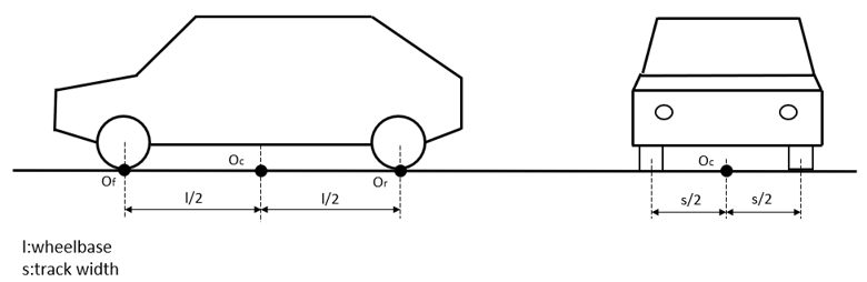
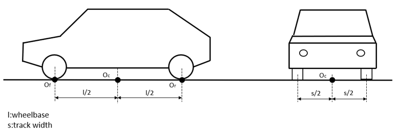
The resultant aerodynamic force and torque is considered to act on a reference point O_c placed on the road surface at the center of the four wheels.

Figure 1.

F_a,x = c_x(τ_L)*P(v_r)

F_a,y = c_y(τ_L)*P(v_r)

F_a,z = c_z(τ_L)*P(v_r)

M_a,x = c_mx(τ_L)*l*P(v_r)

M_a,y = c_my(τ_L)* l*P(v_r)

M_a,z = c_mz(τ_L)* l*P(v_r)

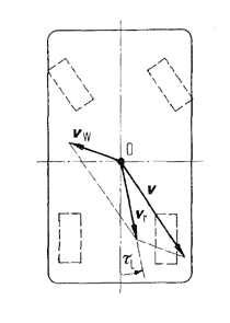
Where c_i express the aerodynamic coefficients, τ_L the relative airflow incidence angle, v_r the resulting velocity, P the dynamic pressure and l the wheelbase.

The coordinate system in which the above defined force and torque components are to be applied is located in O_c and fixed to the car body.

On Velocities

A diagonal airflow results in a flow velocity v_r with an incidence angle τ_L to the vehicle’s longitudinal axis. Both parameters v_r and τ_L can be calculated by vector addition of the road speed vector v (negative car speed vector) and the wind velocity vector v_w.

Figure 2.

On P(v_r)

The dynamic pressure can be calculated using the air density ρ, the resulting velocity v_r, and the following formula.

P(v_r) = 0.5 * ρ * v_r²

The air density is dependent on the ambient temperature and pressure of the environment, and the ideal gas constant for air and it is often regarded as constant.

Vertical Force and Pitch Torque

The vertical force F_a,z and the pitch torque M_a,y are replaced by two vertical forces acting at the center points of the suspensions O_f and O_r at ground level introducing c_z,f and c_z,r.

F_a,zf = c_z,f(τ_L)*P(v_r)

The action forces are applied at reference point O_c placed on the road surface at the center of the four wheels and the center points of the suspensions O_f and O_r at ground level.

Figure 3.

This aerodynamic system is the default setting in the Assembly Wizard for the Car and Truck Library.

The complete set of aerodynamic forces and torques can be applied to the rigid car body as follows:

F_a,x = 0.5*c_x(τ_L)* ρ * A* v_r²

F_a,y = 0.5*c_y(τ_L)* ρ * A* v_r²

F_a,zf = 0.5*c_z,f(τ_L)* ρ * A* v_r²

F_a,zr = 0.5*c_z,r(τ_L)* ρ * A* v_r²

M_a,x = c_mx(τ_L)* l* ρ * A* v_r²

M_a,z = c_mz(τ_L)* l* ρ * A* v_r²

Where A is the frontal area of the car. Vehicle frontal areas are typically in the range of 1.5 m² < A < 2.5 m² for passenger cars and 4 m² < A < 9 m² for trucks and buses.

How to Determine c_i

As a very rough approximation the c_i can be regarded as constants, and to disable aerodynamic totally, all c_i can be set to zero.

One limitation of using this table is that is does not allow situations where the car is subjected to diagonal airflow of over 30 degrees (some of the curves go up to 40 degrees). Such conditions, especially pure sidewind conditions, will be considered for implementation in future releases.

ci coefficients could be derived by a virtual wind tunnel experiment. The values measured in such an experiment would be the constrained forces at O_c, O_r and O_f as functions or v_r and τ.