Magnet (unidirectional): demagnetization curve (HcB, HcJ and Br)

Presentation

This model (Nonlinear magnet described by HcB, HcJ and Br module) defines a nonlinear B(H) dependence. Non-linearity is considered in the direction of magnetization whereas the model's behavior is linear in the transversal directions.

This magnet model is noted as unidirectional because the mathematical model and the direction of magnetization are dissociated (About orientation of magnets). The mathematical model defines the demagnetization curve, while the direction of magnetization is defined by the orientation in the region (Orient materials in massive regions: volume (3D) / face (2D)).

Furthermore, this model can consider demagnetization during solving, wherever the curve knee is, if the corresponding option is selected (Demagnetization during solving).

Mathematical model

The mathematical formula used in Flux for the demagnetization curve is:

This formula is better clarified if we split it into the basic parts.

and

where:

μ₀ is the permeability of vacuum, μ₀ = 4 π 10^-7 (H/m)
B_r is the remanent flux density (T)
H_cJ is the intrinsic coercivity (A/m)
J_s is the saturation magnetic polarization (T)

J_s is automatically computed by Flux when the magnetic field intensity H in the above mathematical formula B(H) is replaced by the normal coercivity -H_cB value.

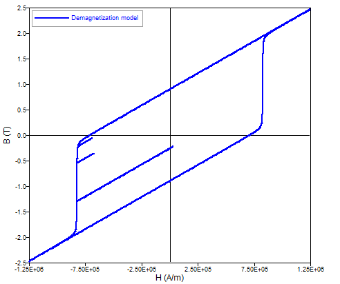
The shape of the B(H) and the J(H) dependence in the direction of magnetization are given in the figure below:

In transversal directions one can write:

where μ_{r ┴} is the transversal relative permeability.

Direction of magnetization

The various possibilities provided to the user are the same ones as those presented in § Magnet (unidirectional): linear approximation.

Demagnetization during solving

With this non-linear model, it is also possible to consider the demagnetization during solving (i.e. the irreversible degradation of a magnet's remanent magnetic flux density due to its interaction with a demagnetizing field) by checking the specific option that is provided during the material creation. This demagnetization model is based on a static Preisach approach and may apply in all quadrants of the magnet B(H) characteristic. The following additional remarks apply:

Available for 2D and 3D in transient magnetic application
In projects containing a magnet material with this option active, it is advisable to set the application to perform an initialization through a static calculation (Application > Transient initialization)
This model does not take in account temperature variations

To use this model in a solved project:

Delete the results;
Go in Application > Edit current application > Transient initialization and select: Initialization by static calculation;
Create a new material Nonlinear magnet described by HcB, HcJ and Br module;
Check the option Taking into account demagnetization during solving;
Assign the material to the regions representing the magnets in the project;
Go to Physics > Face regions (in 2D) or Volume regions (in 3D) > Orient material for face / volume regions to define the direction of magnetization of the magnet;
Solve the scenario.

After solving, to display the current remanent magnetic flux density of a magnet at a given time step:

Select the desired time step;
Create a new Arrows plot, then select the magnet as support;
Then, in the formula editor, click on button Br Magnet (available in the Magnetic Volume region tab) or type BrMagnet (without a space) in the formula field.
Note: In the formula editor, a related button Br is available and the user could also type the corresponding formula Br in the formula field. Remark that these recover the original remanent magnetic flux density stored in the material description, and not the remanent magnetic flux density modified by demagnetization effects at a given time step represented by BrMagnet.

In Flux, hard magnetic materials may be imported, exported and reused with the help of dedicated data exchange tools. These tools are notably useful when used in conjunction with magnets described by the B(H) property of type Nonlinear magnet described by HcB, HcJ and Br module, with the option for consideration of demagnetization during resolution. For a complete discussion on this topic, refer to the following documentation chapter: Import, export and reuse magnets.

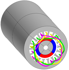
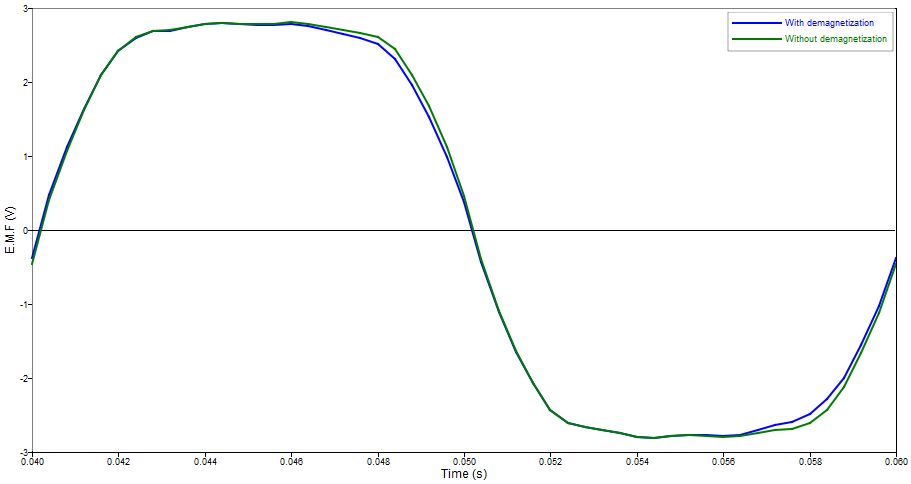
Example of results

Let's consider the permanent magnet motor below, which was represented in a Flux 3D project:

For the control angle values ψ = [0, π/6, π/4, π/3], we can see that there is a local effect on the remanent flux density, which depends on ψ, as shown in the picture below:

Figure 2. Arrow plots of the remanent magnetic flux density of one of the machine's magnet as a function of the control angle ψ.

This localized effect modifies the machine's performance (e.g., torque and back EMF), as illustrated in the picture below.

Figure 3. Back E.M.F with and without demagnetization for ψ = π/4.