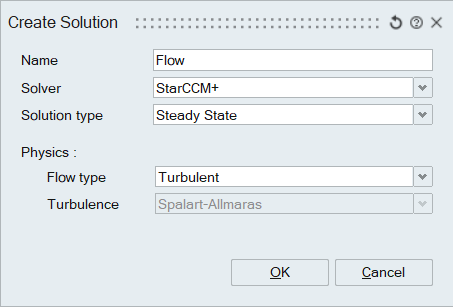
Flow
![]()
Introduction
Flow Solution is used to analyze general fluid flow problems that is used in a wide variety of applications and industries. The flow solver is architected for parallel execution on shared and distributed memory computer systems and provides fast and efficient transient and steady state solutions for standard unstructured element topologies.
A variety of physics is supported including different turbulence models, heat transfer, radiation models, multiphase and moving bodies. You need to select the required physics to be solved in the Solution panel. Accordingly, boundary conditions, solution parameters, material creation and assignment will be setup to run a Flow simulation, launch the solver and visualize the results.
Use SimLab - Learning center videos for more tutorials on Model setup using Solution approach.CFD Mode is supported for flow solution, it displays the entities on which boundary conditions are applied in colors.
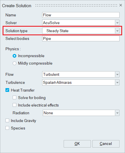
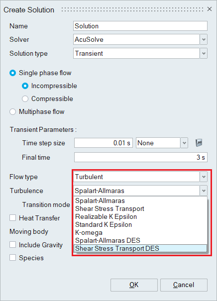
Solution type
Two different Solution types are supported:- Steady State
The time dependence of flow field parameters is an important factor in the analysis of a fluid flow. In a steady state flow, the flow properties at a point, such as pressure and velocity, do not change with time. Steady state flows are of interest in cases where the flow properties need to be studied after the flow field has stabilized.
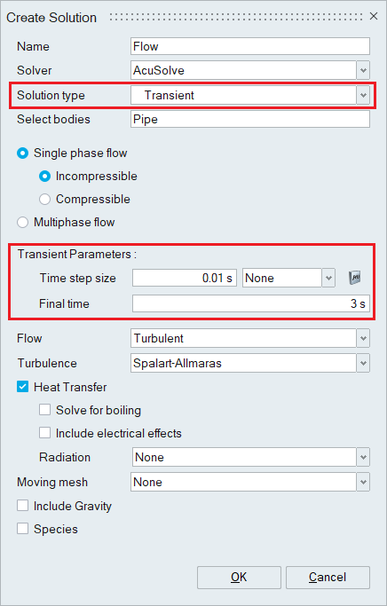
- Transient
If the flow is not steady, then it is said to be unsteady or transient. For a transient simulation, time step size and the total run time needs to be provided. Time step size is the value of time increment made for each time step during a simulation and the Final time is the total physical time the simulation should be performed. Time step size can be ramped up or down during the simulation using a Multiplier Function.
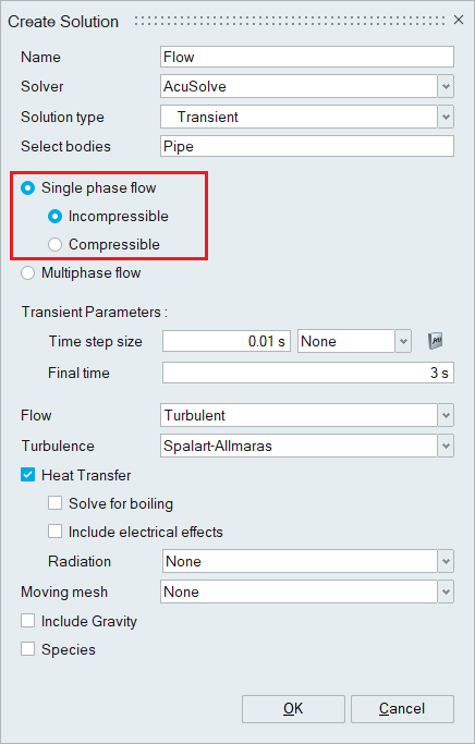
Incompressible flow
Incompressible flow refers to the fluid flow in which the fluid's density is constant. Even though the pressure changes, the density will be constant for an incompressible flow. Incompressible flow means flow with variation of density due to pressure changes is negligible or infinitesimal. All the liquids at constant temperature are incompressible.Compressible/Mildly Compressible flow
Compressible flow deals with flows having significant changes in fluid density. While all flows are compressible, flows are usually treated as being incompressible when the Mach number (the ratio of the speed of the flow to the speed of sound) is smaller than 1.0 (since the density change due to velocity is about 5% in that case). The study of compressible flow is relevant to high-speed aircraft, jet engines, rocket motors, high-speed entry into a planetary atmosphere, gas pipelines, commercial applications such as abrasive blasting, and many other fields.
Select bodies
As the name implies, select the bodies for the simulation. Only the bodies selected will be used for the simulation, even though there are more number of bodies in the SimLab database.
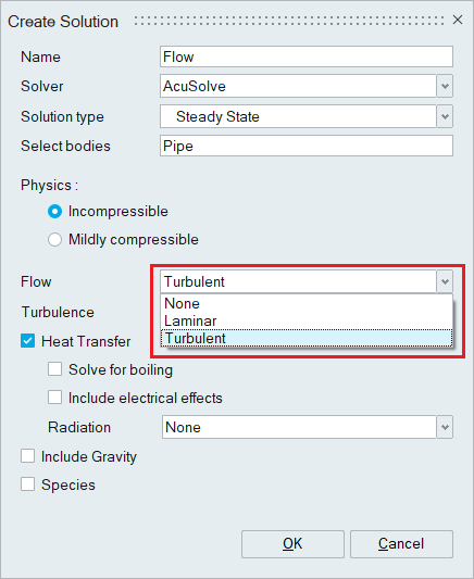
Flow
Flow must be set to None, when there is no flow being modeled in the simulation. This option can be used for Frozen flow simulations where the flow variables are mapped as initial conditions and not solved during the simulation. This option can also be used for modeling heat transfer through solid bodies.
Flow must be set to Laminar,if the fluid motion is characterized by smooth layers and the Reynolds number is within the laminar flow range depending on it is an internal or external flow.
Flow must be set to Turbulent,when the fluid motion is expected to be highly disordered that typically occurs at high velocities and is characterized by velocity fluctuations. Appropriate Turbulent model needs to be selected.
Turbulence
If Flow is set to Turbulent, Turbulence option is displayed. SimLab supports a variety of turbulence models such as Spalart Allmaras, Shear Stress Transport (SST), K-Epsilon and K-Omega. . It also includes Spalart Allmaras DES, and Shear Stress Transport DES for transient analysis. Depending on the problem being solved, an appropriate turbulence model needs to be selected.
Transition mode
Enabling a turbulence transition model allows including the effects of flow transition from laminar to turbulent state. Two transition models namely a) Gamma and b) Gamma Re Theta are supported which are valid for the Spalart-Allmaras, Shear Stress Transport, Spalart-Allmaras DES (detached eddy simulation), and Shear Stress Transport DES turbulence models.
![]()
Heat transfer
Heat Transfer must be activated to perform a thermal analysis. You can just solve only for temperature or you can activate Radiation depending on the problem being solved.
![]()
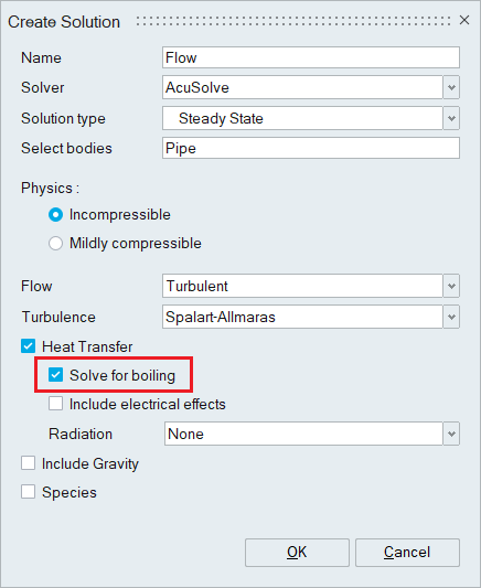
Solve for boiling
If Solve for boiling is activated, single phase nucleate boiling will be modeled using the popular wall heat transfer model for sub-cooled boiling (Steiner Model). A Vapor phase model is required and needs to be provided during material definition.
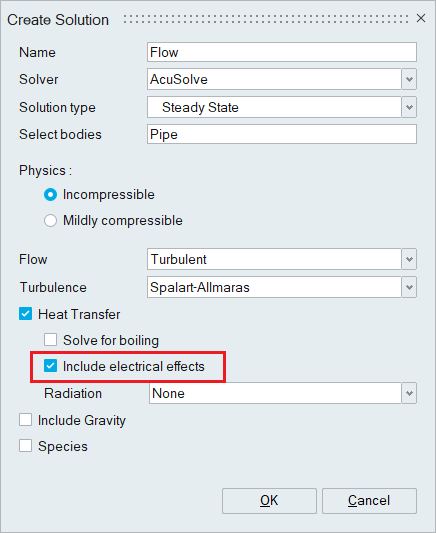
Include electrical effects
If “Include electrical effects” is activated, Joule Heating is modeled. Joule heating is the physical process by which the passage of electrical current through a conducting material produces heat. And electrical energy is converted to thermal energy. Current and Voltage are taken as inputs in the simulation.
- Electronics e.g., fuses, wiring, LEDs
- Battery components e.g., busbars, cells
- Headlamps e.g., LED thermal load
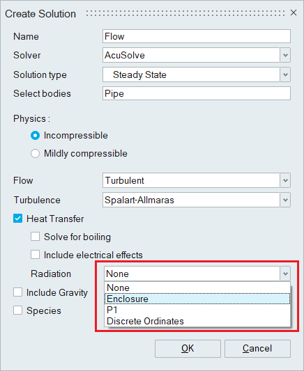
Radiation
Thermal Radiation is the heat transfer caused by the emission of electromagnetic waves carrying energy. This does not require a medium. Radiation is important when there is large temperature difference between surfaces and the environment, and the surfaces have high emissive power (when the emissivity is close to 1 the surface will emit more radiation).
If Heat Transfer option is activated, Radiation option is displayed with the default setting of None. Three different radiation models are supported,
- Enclosure
This model requires a complete enclosure (no hole) and the bodies must be non-participating. Radiation heat fluxes are computed based on the view factors. All the surfaces are assumed to be diffuse and radiation is modeled only on fluid bodies (not on solid bodies).
- P1
This model is more suitable for optically thick media and performs best in scenarios where the radiative intensity is near isotropic. P1 can model both fluid and solid, and in a particular simulation, radiation can be modeled on either a solid or fluid, i.e., there can be only one participating body in a simulation. Also, the surfaces are assumed to be diffuse.
- Discrete Ordinates (DO)
DO radiation model can be used for all optical thicknesses, i.e., non-absorbing and absorbing media. This can model multiple fluid and solid participating bodies in a simulation and supports quadrature’s from S2 – S16 (8-288 directions). Both specular and diffuse surfaces (internal & external) can be modeled.
When and why to choose a specific Radiation Model
| Enclosure | P1 Model | Discrete Ordinates |
|---|---|---|
| Non-participating media | Computationally very efficient – fastest radiation model on offer | High accuracy in arbitrary 3D configurations |
| Not too complex surface configuration; very expensive for many radiation surfaces | Can have lower accuracy for optically thin media | S4 and S6 quadratures are sufficient for many complex 3D problems; quadratures up to S16 are available |
| Surfaces are diffused | Surfaces are diffused | Surfaces are diffused or specular |
| Symmetry boundary condition can be inaccurate | Moving Mesh | No limitations of boundary conditions |
| Moving Mesh |
Multiphase
In general, multiphase flow are mainly observed in real life environment consisting of two or more fluids (gas, liquid, or solid). They have possible combinations of gas-liquid (dissolved gas), liquid-liquid (oil in water), liquid-solid (immersed particles), as well as gas-liquid-solid. Multiphase flow is valid only for transient analysis.
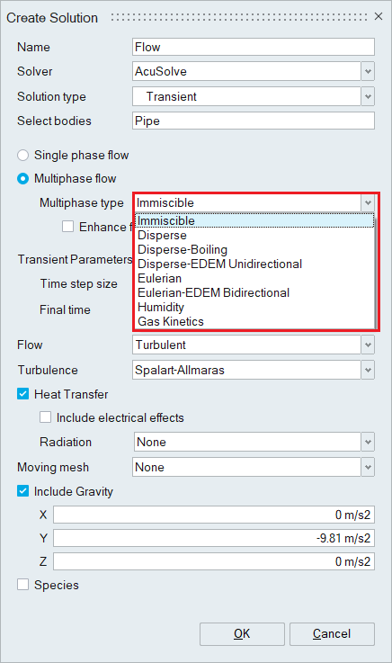
Immiscible
The Immiscible option uses the level set method to capture the interface between immiscible fluids. This type of technology is useful for tracking the interface between fluids for applications such as fuel sloshing in a fuel tank, waves on the surface of the ocean, or a liquid being poured into a container. Two options are available for immiscible multiphase simulations,- Immiscible
- Immiscible with Enhanced Interface Tracking
Both approaches rely on two additional staggers to track the interface. In the standard Immiscible method, the first stagger governs the transport of the interface, and the second stagger controls the sharpness of the interface.
The Immiscible with Enhanced Feature Capturing method includes extra stagger iterations to reduce the amount of diffusion in the solution field. This method captures multiphase interfaces more sharply than the standard Immiscible method. Because more calculations are performed, more computing time is needed when compared to the standard Immiscible method.

Disperse
The Disperse option is used to simulate multiple-dispersed fields with one carrier fluid. The dispersed fields (particles, bubbles, droplets) are tracked as Eulerian fields while calculating the momentum exchange between the dispersed fields and the carrier using an algebraic slip model. In general, it is recommended that the heavier fluid is specified as the carrier. For the case where the dispersed field and carrier field are separated, the Algebraic Eulerian method tracks the interface as a smooth interface between fluids. Unlike the Immiscible (level set) approach, an additional stagger is not needed to track the interface. Solver solves the mixture continuity, mixture momentum equations and field volume fraction equations.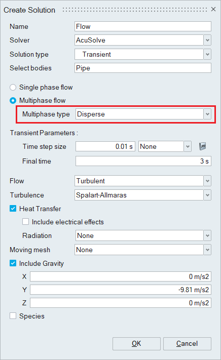
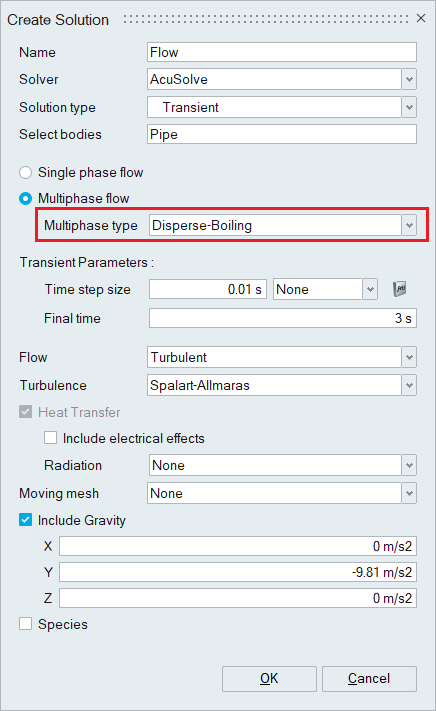
- Disperse-Boiling
For the Disperse-Boiling type, phase change for the disperse multiphase is activated. Nucleate boiling by the heated wall is modeled with RPI wall boiling model. This is also called the multiphase nucleate boiling.
- Eulerian
Eulerian multiphase gives you the capability to simulate interactions between continuous or disperse fields. The carrier must be a fluid and the disperse phases can either be fluids (gas, vapor, bubbles) or solids. SimLab allows up to 5 disperse phases and the interactions between multiple disperse phases is not supported (only interaction between carrier and disperse phases is supported).
The basic assumption of disperse multiphase approach is that the disperse phase is accelerated to a terminal velocity in a short distance. If this assumption is no longer valid, then Eulerian multiphase should be used.

- Disperse-EDEM Unidirectional
- Eulerian-EDEM Bidirectional
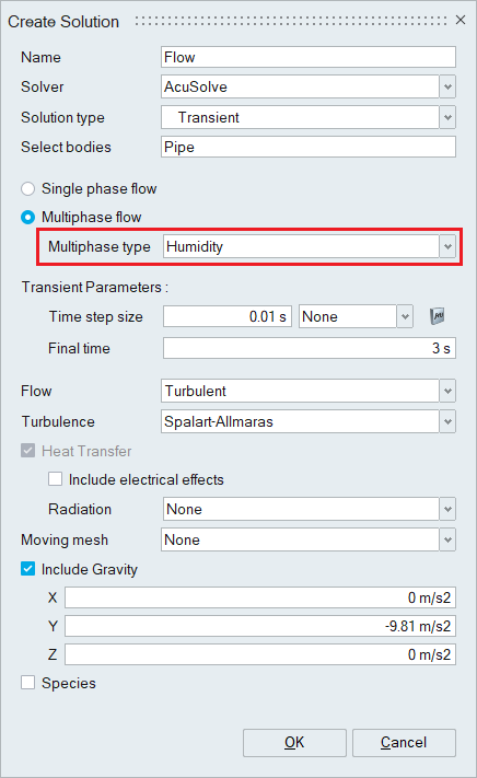
- Humidity
When using the Humidity, solver tracks the spread of “Water vapor” field by solving the field's mass fractions equation in the form of species transport equation in addition to solving the mixture continuity, momentum equations and energy equations.
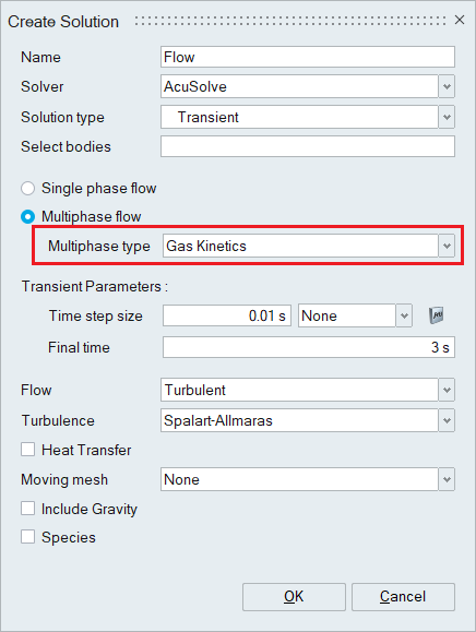
- Gas Kinetics
The Gas Kinetics model account for molecular configuration and weight, intermolecular energies collision, and other parameters to predict the proper advection, diffusion, and blending of the various gases. Evaluation of pure species properties follows standard kinetic theory expressions and one can choose from a range of possibilities for evaluating mixture properties.
SimLab currently supports 5 gases namely Oxygen, Nitrogen, Hydrogen, Methane, and Propane.
Moving Mesh
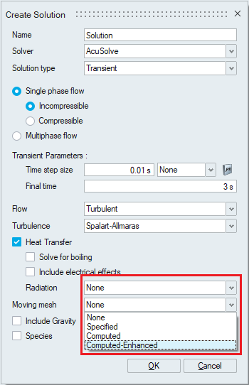
Three types of mesh motion options are supported,
- None - The mesh is fixed in the simulation. There will not be any moving bodies in the simulation.
- Specified - Mesh motion must be provided as an input in the simulation. Examples are rotational speed input for blowers and fans.
- Computed - Mesh motion is computed by the solver using Arbitrary Lagrangian Eulerian (ale) technology.
- Computed -Enhanced - Enhanced arbitrary mesh movement useful for extreme mesh deformation cases.
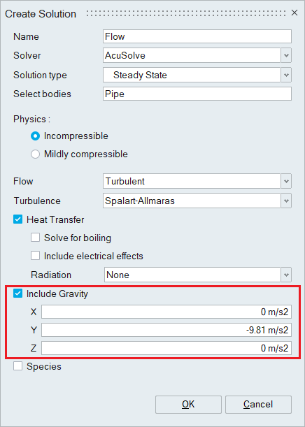
Gravity
A global value of gravitational acceleration can be set and applied to all the bodies in the simulation.
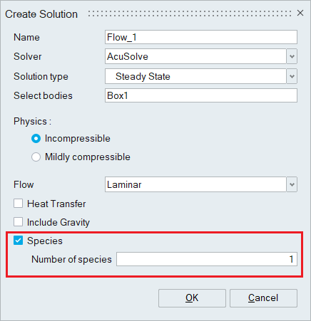
Species
Species are passive scalars that allow to simulate the transport of a scalar quantity. SimLab currently supports up to 9 species. The Species flag enables the solving of passive scalars and Users can define the number of species to be modelled in the simulation.
CAD-based solution
- Analysis > Advanced > Advanced BC
- Analysis > Advanced > Periodic
- Analysis > Mesh Motion > Displacement
- Analysis > Interface Surface
- Analysis > Components > Contact Resistance
Supported solvers
| Solver | Analysis |
|---|---|
| AcuSolve |
|
| OpenFOAM |
|
| StarCCM+ | Steady |
StarCCM++
For StarCCM++, only mesh export is supported. The mesh can be exported using the following methods,
- STL - Exports surface meshes or surfaces derived from solid meshes into a single file.
- CGNS - Supports export of volume meshes only.
Using these methods, body and surface names are preserved upon import into STAR-CCM++.