Response Spectrum Analysis

Response Spectrum Analysis (RSA) is a technique used to estimate the maximum response of a structure for a transient event. Maximum displacement, stresses, and/or forces may be determined in this manner.

The technique combines response spectra for a specified dynamic loading with results of a normal modes analysis. The time-history of the responses are not available.

Response spectra describes the maximum response versus natural frequency of a 1-DOF system for a specified dynamic loading. They are employed to calculate the maximum modal response for each structural mode. These modal maxima may then be combined using various methods, such as the Absolute Sum (ABS) method or the Complete Quadratic Combination (CQC) method, to obtain an estimate of the peak structural response.

RSA is a simple and computationally inexpensive method to provide an approximation of peak response, compared to conventional transient analysis. The major computational effort is to obtain a sufficient number of normal modes in order to represent the entire frequency range of input excitation and resulting response. Response spectra are usually provided by design specifications; given these, peak responses under various dynamic excitations can be quickly calculated. Therefore, it is widely used as a design tool in areas such as seismic analysis of buildings.

Governing Equations

Normal Modes Analysis

The equilibrium equation for a structure performing free vibration appears as the eigenvalue problem:

(K - λ M) A = 0

Where,

$K$: Stiffness matrix of the structure.
$M$: Mass matrix.; Damping is neglected.

The solution of the eigenvalue problem yields $n$ eigenvalues $λ_{i}$ , where $n$ is the number of degrees of freedom. The vector $A$ is the eigenvector corresponding to the eigenvalue.

The eigenvalue problem is solved using the Lanczos or the AMSES method. Not all eigenvalues are required and only a small number of the lowest eigenvalues are normally calculated. The results of eigenvalue analysis are the fundamentals of response spectrum analysis.

Response spectrum analysis can be performed together with normal modes analysis in a single run, or eigenvalue analysis with Lanczos solver can be performed first to save eigenvalues and eigenvectors by using EIGVSAVE, which can be retrieved later by using EIGVRETRIEVE for response spectrum analysis.

Modal Combination

It is assumed each individual mode behaves like a single degree-of-freedom system. The transient response at a degree of freedom is:

u_{k} = \sum_{i} A_{i k} ψ_{i} χ

Where,

$A$: Eigenvector
$ψ$: Modal participation factor
$χ$: Response spectrum

For loading due to base acceleration, the modal participation factor can be expressed as:

ψ_{i} = A_{i}^{T} M T

Where,

$A$: Eigenvector
$M$: Mass matrix
$T$: Rigid body motion due to excitation

In ABS modal combination, the peak response is estimated by:

u_{k} = \sum_{i} | A_{i k} | | ψ_{i} χ |

In CQC modal combination, the peak response is estimated by:

u_{k} = \sqrt{\sum_{m} \sum_{n} v_{m} ρ_{m n} v_{n}}

Where,

$v_{m}$: $m^{t h}$ mode's contribution to $u_{k}$ ; equal to $A_{m k} ψ_{k} χ$ .
$ρ_{m n}$: Cross-modal coefficient

The cross modal coefficient $ρ_{m n}$ between modes $m$ and $n$ is calculated as:

ρ_{m n} = \frac{8 \sqrt{ξ_{m} ξ_{n}} (ξ_{m} + r_{n m} ξ_{n}) r_{n m}^{1.5}}{{(1 - r_{n m}^{2})}^{2} + 4 ξ_{m} ξ_{n} r_{n m} (1 + r_{n m}^{2}) + 4 (ξ_{m}^{2} + ξ_{n}^{2}) r_{n m}^{2}}

Where,

$r_{n m} = \frac{λ_{n}}{λ_{m}}$: Ratio of eigenvalues of the modes
$ξ_{m} and ξ_{n}$: Modal damping values of the two modes

In SRSS modal combination, the peak response is estimated by:

u_{k} = \sqrt{\sum_{i} {(A_{i k} ψ_{i} χ)}^{2}}

The SRSS method is less conservative than ABS method. It is more accurate when the modes are well separated.

The NRL method combines ABS and SRSS methods. It adds the maximum modal response by ABS method and the rest of the modes by SRSS method. The peak response is estimated by:

u_{k} = | A_{i k} | | ψ_{i} χ | + \sqrt{\sum_{j \neq i} {(A_{j k} ψ_{j} χ)}^{2}}

Directional Combination

In order to estimate peak response due to dynamic excitations in different directions, the peak response in each direction must be combined to obtain total peak response. Methods such as ALG (algebraic) and SRSS (square root of sum of squares) can be used.

Missing Mass Response

Response spectrum analysis typically involves using a limited number of dynamic modes to represent the structural behavior. This approach involves exclusion of high-frequency modes or rigid modes in the modal summation.

Hence the mass associated with these high-frequency modes needs to be accounted for. Since the high frequency modes do not have dynamic amplification, it is feasible to estimate the missing mass response by using a pseudo-static analysis. In this analysis, a pseudo-static loading is applied which is equal to the missing inertia force of the high frequency modes, calculated as:

F_{M} = M (\sum_{j = 1}^{N} A_{j} ψ_{j} - T) S_{a 0}

Where,

$S_{a 0}$: Zero periodic acceleration (ZPA).
$F_{M}$: Missing inertia force of high frequency modes.

The missing mass response is then obtained by performing a linear static analysis under the pseudo loading.

R_{M} = K^{-1} F_{M}

Where,

$R_{M}$: Missing mass response.
$K$: Structural stiffness.

The missing mass response can be combined with the known modal responses with SRSS method.

R_{a} = \sqrt{\sum_{i = 1}^{N} \sum_{j = 1}^{N} ε_{i j} R_{i} R_{j} + R_{M}^{2}}

Where,

$ε_{i j}$: Modal combination coefficient.
$R_{i}$ / $R_{j}$: Modal response of the i/j mode.
$R_{a}$: Total response.

Rigid Response

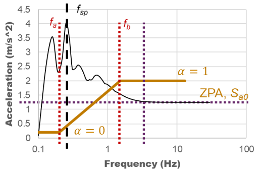
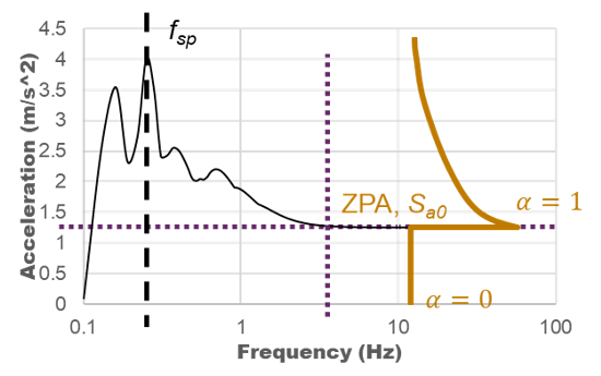
The modal response can be divided into periodic part and rigid part by introducing a coefficient α.

Rigid part:

R_{r i} = α_{i} R_{i}

Periodic part:

R_{p i} = \sqrt{1 - α_{i}^{2}} R_{i}

Where,

$R_{r i}$: Rigid part of modal response.
$R_{p i}$: Periodic part of modal response.
$α_{i}$: Ratio of rigid part to the modal response.

When α is zero, the response is a pure periodic response. When α is one, it is a pure rigid response. The coefficient α can be estimated by using Gupta method or Lindley-Yow method.

Gupta method calculates α based on the frequency. When the frequency is less than a frequency limit fa, α = 0; When the frequency is greater than the frequency limit fb, α = 1; When the frequency is between fa and fb, α is calculated as:

α_{i} = \frac{\ln (\frac{f_{i}}{f_{a}})}{\ln (\frac{f_{b}}{f_{a}})}

Lindley-Yow method calculates α based on the acceleration response spectrum value. When the spectrum value is equal to ZPA, α = 1; When the spectrum value is less than ZPA, α = 0; When the spectrum value is greater than ZPA, α is calculated as:

α_{i} = \frac{S_{a 0}}{S_{a i}}

The total response considering both rigid response and missing mass response can be calculated with the following formula. Missing mass response is a part of rigid response. The periodic response and rigid response are combined with SRSS method.

R_{a} = \sqrt{\sum_{i = 1}^{N} \sum_{j = 1}^{N} ε_{i j} \sqrt{1 - α_{i}^{2}} R_{i} \sqrt{1 - α_{j}^{2}} R_{j} + {(\sum_{i = 1}^{N} α_{i} R_{i} + R_{M})}^{2}}

Input Specification

Subcase Definition

An RSA subcase may be explicitly identified by setting ANALYSIS=RSPEC, but it is also implicitly chosen for any subcase containing the RSPEC data selector (when the ANALYSIS entry is not present).

The following data selectors are recognized for an RSA subcase definition.

METHOD: References an eigenvalue extraction Bulk Data Entry definition (EIGRL). Only METHOD(STRUCTURE) is supported. This reference is required.
RSPEC: References an RSPEC Bulk Data Entry where the combination rules and the input spectra are identified. This reference is required.
SDAMPING: References damping table Bulk Data Entries (TABDMP1 or TABDMP2) to specify modal damping. This reference is required.
SPC: References single point constraint Bulk Data Entries (SPCADD, SPC and SPC1).
MPC: References multi-point constraint Bulk Data Entries (MPCADD or MPC).
STATSUB(PRELOAD): Pre-loading is supported for a Response Spectrum analysis subcase. STATSUB(PRELOAD) can be used to identify the subcase used to apply the preloading. The eigenvalues are augmented with the pre-loading effect coming from the pre-loading subcase.

Bulk Data

Bulk Data Entries which have particular significance for RSA include:

RSPEC: Specifies combination rules, excitation DOF, and references the input spectra.
DTI,SPECSEL: Defines response spectra.
EIGRL: Defines parameters for eigenvalue extraction.
PARAM, LFREQ and PARAM, HFREQ: Defines the range of modes used in modal combinations.
TABDMP1: Specifies modal damping as a function of frequency.
TABDMP2: Specifies modal damping as a function of a range of mode indices.
SPC, SPC1, and SPCADD: Specifies base where excitation is applied and other constraints.

Example: Input

SUBCASE 100
	RSPEC = 2
	SPC = 5
	SDAMPING = 12
	METHOD = 24
$
BEGIN BULK
$
PARAM, LFREQ, 0.1
PARAM, HFREQ, 1000.
EIGRL, 24, 0.0, 1000.
RSPEC, 2, ABS, CQC, 0.1
, 99, 2.0, 1.0, 0.0, 0.0
DTI, SPECSEL, 99, , A, 2, 0., 3, 0.02,
, 4, 0.04, ENDREC
TABDMP1, 12, …
TABLED1, 2
+,…
TABLED1, 3
+,…
TABLED1, 4
+,…
ENDDATA
$

Output

Results of interest from RSA include maximum displacement, stress, strain, force, and section forces. These are requested via the I/O Options Entry DISPLACEMENT, STRESS / ELSTRESS, STRAIN, FORCE / ELFORCE, and RESULTANT respectively. Neuber correction is also supported for STRESS and STRAIN outputs in response spectrum analysis. More details on the supported output formats for the results can be found in Results Output by OptiStruct.

For shell elements, corner stresses are available in the H3D, PCH and OP2 file formats, while corner strains are available in the OP2 file format. For more information on the location of element outputs, refer to STRESS and STRAIN in the Reference Guide.

For bar and beam elements defined using PBARL and PBEAML respectively in RSA, von Mises Stress output is available in the .h3d file format.