Rotor Dynamics

Rotor Dynamics is the analysis of structures containing rotating components.

The dynamic behavior of such structures is influenced by the type and angular velocity of rotating components and their locations within the model. Rotor dynamics is available in OptiStruct for modal frequency response, complex eigenvalue, static, linear direct transient and small displacement nonlinear direct transient analyses.

OptiStruct supports both 1D and 3D rotors for Rotor Dynamic Analysis.

Motivation

When a component within the structure rotates, additional forces like the gyroscopic force and circular damping force act on it. It is important to determine the effects of rotating components on the system as a whole. The natural frequencies of a system usually change, if gyroscopic forces act on the model due to a rotating component. Circulating damping forces due to rotating components can lead to system instability. These forces are a function of the frequency of rotating component. In OptiStruct, they are included in the calculation of the response of the structure of interest when required in applicable subcases.

Figure 1. Application of Rotor Dynamics Analysis

In Figure 1, the rotating components of the structure are the shafts on which gears are mounted. The design of the rotors and their angular frequencies can affect the dynamic response of the structure. Any design will most likely lead to asymmetrical mass distribution about the rotor axes. This unbalanced mass, even if it is not significant, can result in deflection of the rotor depending on various factors. The magnitude of these deflections will be augmented when the rotating speed of the shafts equals the natural frequency of the structure (Resonance), and can lead to catastrophic failure of the system.

Implementation

The Rotor Dynamics functionality is activated in OptiStruct with the use of the RGYRO Subcase Information Entry (RGYRO=ID). This RGYRO entry references the identification number of a RGYRO Bulk Data Entry. Related Bulk Data Entries, RSPINR, UNBALNC, ROTOR/ROTORG and RSPEED are defined in the model for Rotor Dynamics. Parameters PARAM,GYROAVG, PARAM,WR3, and PARAM,WR4 are also used.

Whirl

A rotor is a structure that rotates about its own axis at a specific angular velocity. If a lateral force is applied to the rotor, it will deform in the lateral direction. This deformation is dependent on various factors, such as, magnitude of the applied force, rotor material properties, stator stiffness, and damping within the system. Due to rotor rotation, the deformed rotor will also whirl about an axis.

Synchronous and Asynchronous Analysis

The whirling speed can either be the same as rotor speed or it can be different from it. The type of analysis performed if the whirling speed and the rotor speed match is known as synchronous analysis. If the speeds do not match, then asynchronous analysis is used to determine the dynamic response of the model. In OptiStruct, the RGYRO Bulk Data Entry can be used to select synchronous/asynchronous analysis.

Figure 2. Types of Whirl and the Two Analysis Types that are Dependent on the Angular Frequency of a Rotor

Forward Whirl and Backward Whirl

The type of whirl depends on the spin direction of a rotor. If the rotor spin direction is the same as that of its whirl direction, then it is termed as forward whirl. If the rotor spin direction is opposite to the whirl direction, it is termed as backward whirl. In complex eigenvalue analysis, you can determine and differentiate between the modes of a structure undergoing backward whirl and forward whirl.

Supported Solution Sequences

OptiStruct supports the Rotor Dynamics functionality in the following solution sequences.

Frequency Response Analysis

The response of a structure with rotating components to a specified external excitation can be determined using the rotor dynamics functionality in frequency response analysis.

Asynchronous Analysis (RGYRO=ASYNC)

If ASYNC is specified in the RGYRO Bulk Data Entry, the rotors within the structure have user-defined spin rates. The excitation frequency (FREQi Bulk Data Entries) is independent of the reference rotor speed defined in the RGYRO Bulk Data Entry.

Synchronous Analysis (RGYRO=SYNC)

If SYNC is specified in the RGYRO Bulk Data Entry, the reference rotor spin rate is equal to (or synchronous with) the excitation frequency. The reference rotor speed is not input via the RGYRO Bulk Data Entry and the FREQi Bulk Data Entries values are used in this analysis.

Complex Eigenvalue Analysis

The eigenvalues and critical speeds of a structure with rotating components can be determined using the rotor dynamics functionality in complex eigenvalue analysis.

Asynchronous Analysis (RGYRO=ASYNC)

If ASYNC is specified in the RGYRO Bulk Data Entry, the rotors within the structure have user-defined spin rates via the RSPEED entry and the Campbell Diagram can be plotted to find the critical speeds. Additionally, since the calculated eigenvalues are complex, you can determine unstable modes by studying the real parts of the calculated eigenvalues. If the real part of a complex eigenvalue is positive, then the corresponding system mode is unstable.

Synchronous Analysis (RGYRO=SYNC)

If SYNC is specified in the RGYRO Bulk Data Entry, only the critical speeds are calculated as the rotor speeds are equal to the whirl frequencies. These critical speeds can lead to structural resonance and the design should be modified to change its whirl frequencies or the operating rotor spin rate should be limited to avoid reaching the critical speeds.

Note: In a Frequency Response Analysis, the Synchronous Analysis (SYNC) option is generally used to model rotors with an inherent unbalance. The rotor unbalance can be specified as a force or via the UNBALNC Bulk Data Entry. The analysis is synchronous because the unbalanced load vibrates at the whirl frequency of the system which is equal to the rotor spin speed.

Frequency Response Analysis (ASYNC)

Asynchronous Analysis is activated using the RGYRO=ASYNC option. Frequency Response Analysis in rotor dynamics involves defining the excitation either as an external varying load as a function of frequency or as a rotor unbalance via the UNBALNC Bulk Data Entry (or as a force that simulates the effect of the rotor unbalance). Asynchronous frequency response analysis in OptiStruct is designed for an external varying force at a specific set of frequencies. The following equation implements the external loading functionality in OptiStruct. The rotor speeds should be specified by you for Asynchronous Frequency Response Analysis.

(\begin{array}{l} - ω^{2} M + i ω (C_{S} + α_{s 1} M_{S} + α_{s 2} K_{S} + C_{S H}) + (1 + i G) K_{S} + i C_{S M} + i C_{S H M} \\ + \sum_{j = 1}^{N} (\begin{array}{l} (1 + i {(G R)}_{j}) {(K_{R})}_{j} + i {(C_{R M})}_{j} + i {(C_{R H M})}_{j} + i ω {(α_{R 1} M_{R} + α_{R 2} K_{R} + C_{R} + C_{R H})}_{j} \\ + {(Ω_{R})}_{j} (\begin{array}{l} i ω {(C_{R G})}_{j} + {(C_{R}^{C})}_{j} + {(C_{R H}^{C})}_{j} + {(α_{R 1} M_{R}^{C} + α_{R 2} K_{R}^{C})}_{j} \\ + \frac{G R}{ω} {(K_{R}^{C})}_{j} + \frac{1}{ω} ({(C_{R H M}^{C})}_{j} + {(C_{R M}^{C})}_{j}) \end{array}) \end{array}) \end{array}) u (ω) = f (ω)

The response of a system with rotating components to an external load in the frequency domain is calculated based on Equation 1.

Frequency Response Analysis (SYNC)

Synchronous Analysis is activated using the RGYRO=SYNC option. Frequency Response Analysis in rotor dynamics involves defining the excitation either as an external varying load as a function of frequency or as a rotor unbalance via the UNBALNC Bulk Data Entry (or as a force that simulates the effect of the rotor unbalance). Synchronous Frequency Response Analysis in OptiStruct is designed to calculate the response of a system with a rotor unbalance. The following equation implements the rotor unbalance functionality in OptiStruct. The rotor speeds are determined from the FREQi entries for Synchronous frequency response analysis.

(\begin{array}{l} - Ω_{r e f}^{2} (M - i \sum_{j = 1}^{N} β_{j} {(C_{R G})}_{j}) + i Ω_{r e f} (C_{S} + α_{s 1} M_{S} + α_{s 2} K_{S} + C_{S H}) + (1 + i G) K_{S} + i C_{S M} + i C_{S H M} \\ + \sum_{j = 1}^{N} (\begin{array}{l} (1 + i {(G R)}_{j}) {(K_{R})}_{j} + i {(C_{R M})}_{j} + i {(C_{R H M})}_{j} + i Ω_{r e f} {(α_{R 1} M_{R} + α_{R 2} K_{R} + C_{R} + C_{R H})}_{j} \\ + (α_{j} + Ω_{r e f} β_{j}) (\begin{array}{l} + i Ω_{r e f} α_{j} {(C_{R G})}_{j} + {(C_{R}^{C})}_{j} + {(C_{R H}^{C})}_{j} + {(α_{R 1} M_{R}^{C} + α_{R 2} K_{R}^{C})}_{j} \\ + \frac{G R}{Ω_{r e f}} {(K_{R}^{C})}_{j} + \frac{1}{Ω_{r e f}} ({(C_{R H M}^{C})}_{j} + {(C_{R M}^{C})}_{j}) \end{array}) \end{array}) \end{array}) u (Ω_{r e f}) = f (Ω_{r e f})

The response of a system with rotating components to a rotor imbalance which is considered as a force acting in the frequency domain is calculated based on Equation 2.

Frequency Response Analysis with WR3, WR4 and WRH (ASYNC)

Parameters PARAM,WR3, PARAM,WR4, and PARAM,WRH can be used to avoid frequency dependent calculation of the rotor damping and circulation terms in systems with multiple rotors. The frequency values in the circulation damping terms are replaced with the values of the parameters as shown in Equation 3. PARAM,GYROAVG should be set to -1 to be able to bypass frequency dependent look-up and use the WR3, WR4, and WRH values.

(\begin{array}{l} - ω^{2} M + i ω (C_{S} + α_{s 1} M_{S} + α_{s 2} K_{S} + C_{S H}) + (1 + i G) K_{S} + i C_{S M} + i C_{S H M} \\ + \sum_{j = 1}^{N} (\begin{array}{l} (1 + i ω (\frac{G R}{W R 3})) {(K_{R})}_{j} + i ω (\frac{1}{W R 4}) {(C_{R M})}_{j} + i ω (\frac{1}{W R H}) {(C_{R H M})}_{j} \\ + i ω {(α_{R 1} M_{R} + α_{R 2} K_{R} + C_{R} + C_{R H})}_{j} \\ + {(Ω_{R})}_{j} (\begin{array}{l} i ω {(C_{R G})}_{j} + {(C_{R}^{C})}_{j} + {(C_{R H}^{C})}_{j} + {(α_{R 1} M_{R}^{C} + α_{R 2} K_{R}^{C})}_{j} \\ + \frac{G R}{W R 3} {(K_{R}^{C})}_{j} + \frac{1}{W R 4} {(C_{R M}^{C})}_{j} + \frac{1}{W R H} {(C_{R H M}^{C})}_{j} \end{array}) \end{array}) \end{array}) u (ω) = f (ω)

Frequency Response Analysis with WR3, WR4 and WRH (SYNC)

Parameters PARAM,WR3, PARAM,WR4 and PARAM,WRH can be used to avoid frequency dependent calculation of the rotor damping and circulation terms in systems with multiple rotors. The rotor speeds can be calculated as a linear function of the reference rotor spin rate (see description of terms below). The reference rotor spin rate values in the circulation damping terms are replaced with the values of the parameters as shown in Equation 4. PARAM,GYROAVG should be set to -1 to be able to bypass frequency dependent look-up and use the WR3, WR4, and WRH values.

(\begin{array}{l} - Ω_{r e f}^{2} (M - i \sum_{j = 1}^{N} β_{j} {(C_{R G})}_{j}) + i Ω_{r e f} (C_{S} + α_{s 1} M_{S} + α_{s 2} K_{S} + C_{S H}) + (1 + i G) K_{S} + i C_{S M} + i C_{S H M} \\ + \sum_{j = 1}^{N} (\begin{array}{l} {(K_{R})}_{j} + i Ω_{r e f} \frac{G R}{W R 3} {(K_{R})}_{j} + i Ω_{r e f} \frac{1}{W R 4} {(C_{R M})}_{j} + i Ω_{r e f} \frac{1}{W R H} {(C_{R H M})}_{j} \\ + i Ω_{r e f} α_{j} {(C_{R G})}_{j} + i Ω_{r e f} {(α_{R 1} M_{R} + α_{R 2} K_{R} + C_{R} + C_{R H})}_{j} \\ + (α_{j} + Ω_{r e f} β_{j}) (\begin{array}{l} {(C_{R}^{C})}_{j} + {(C_{R H}^{C})}_{j} + {(α_{R 1} M_{R}^{C} + α_{R 2} K_{R}^{C})}_{j} \\ + \frac{G R}{W R 3} {(K_{R}^{C})}_{j} + \frac{1}{W R H} {(C_{R H M}^{C})}_{j} + \frac{1}{W R 4} {(C_{R M}^{C})}_{j} \end{array}) \end{array}) \end{array}) u (Ω_{r e f}) = f (Ω_{r e f})

Complex Eigenvalue Analysis with WR3, WR4 and WRH (ASYNC)

The eigenvalues and critical speeds of a structure with rotating components can be determined using the rotor dynamics functionality in Complex Eigenvalue Analysis. In Asynchronous Analysis the critical speeds can also be determined by plotting the Campbell diagram for frequencies specified using the RSPEED Bulk Data Entry. The parameters PARAM,WR3, PARAM,WR4, and PARAM,WRH can be used to replace the values of WR3, WR4, and WRH in Equation 5.

(\begin{array}{l} - ω^{2} M + i ω (C_{S} + α_{s 1} M_{S} + α_{s 2} K_{S} + C_{S H}) + (1 + i G) K_{S} + i C_{S M} + i C_{S H M} \\ + \sum_{j = 1}^{N} (\begin{array}{l} (1 + i ω (\frac{G R}{W R 3})) {(K_{R})}_{j} + i ω (\frac{1}{W R 4}) {(C_{R M})}_{j} + i ω (\frac{1}{W R H}) {(C_{R H M})}_{j} \\ + i ω {(α_{R 1} M_{R} + α_{R 2} K_{R} + C_{R} + C_{R H})}_{j} \\ + {(Ω_{R})}_{j} (\begin{array}{l} i ω {(C_{R G})}_{j} + {(C_{R}^{C})}_{j} + {(C_{R H}^{C})}_{j} + {(α_{R 1} M_{R}^{C} + α_{R 2} K_{R}^{C})}_{j} \\ + \frac{G R}{W R 3} {(K_{R}^{C})}_{j} + \frac{1}{W R 4} {(C_{R M}^{C})}_{j} + \frac{1}{W R H} {(C_{R H M}^{C})}_{j} \end{array}) \end{array}) \end{array}) u (ω) = 0

Complex Eigenvalue Analysis with WR3, WR4 and WRH (SYNC)

Only the rotor speeds are required to perform the Synchronous Complex Eigenvalue Analysis as the whirl frequencies are equal to the reference rotor spin rates. Only the critical speeds are output as a result of this analysis. The parameters PARAM,WR3, PARAM,WR4, and PARAM,WRH can be used to replace the values of WR3, WR4, and WRH in Equation 6.

(\begin{array}{l} - Ω_{r e f}^{2} (M - i \sum_{j = 1}^{N} β_{j} {(C_{R G})}_{j}) + i Ω_{r e f} (C_{S} + α_{s 1} M_{S} + α_{s 2} K_{S} + C_{S H}) + (1 + i G) K_{S} + i C_{S M} + i C_{S H M} \\ + \sum_{j = 1}^{N} (\begin{array}{l} {(K_{R})}_{j} + i Ω_{r e f} (\begin{array}{l} \frac{G R}{W R 3} {(K_{R})}_{j} + \frac{1}{W R 4} {(C_{R M})}_{j} + \frac{1}{W R H} {(C_{R H M})}_{j} + α_{j} {(C_{R G})}_{j} \\ + {(α_{R 1} M_{R} + α_{R 2} K_{R} + C_{R} + C_{R H})}_{j} \end{array}) \\ + (α_{j} + Ω_{r e f} β_{j}) (\begin{array}{l} {(C_{R}^{C})}_{j} + {(C_{R H}^{C})}_{j} + {(α_{R 1} M_{R}^{C} + α_{R 2} K_{R}^{C})}_{j} \\ + \frac{G R}{W R 3} {(K_{R}^{C})}_{j} + \frac{1}{W R H} {(C_{R H M}^{C})}_{j} + \frac{1}{W R 4} {(C_{R M}^{C})}_{j} \end{array}) \end{array}) \end{array}) u (Ω_{r e f}) = 0

Static

For Static Analysis, the following moment term is added to the load vector at each rotor grid.

f = - \sum_{j = 1}^{N} Ω_{j} {(C_{R G})}_{j} \vec{ω}

Linear and Small Displacement Nonlinear Direct Transient Analysis

The rotor speeds ( $Ω$ ) are time-dependent in Transient Rotor Dynamics. The displacement equation (with WR3, WR4, and WRH) is:

\begin{array}{l} M \ddot{u} (t) + \dot{u} (t) (\begin{array}{l} C_{S} + α_{s 1} M_{S} + α_{s 2} K_{S} + C_{S H} + (\frac{G}{W 3}) K_{S} + (\frac{1}{W 4}) C_{S M} + (\frac{1}{W H}) C_{S H M} \\ + \sum_{j = 1}^{N} (\begin{array}{l} {(α_{R 1} M_{R} + α_{R 2} K_{R})}_{j} + {(C_{R})}_{j} + {(C_{R H})}_{j} + (\frac{G R_{j}}{W R 3}) {(K_{R})}_{j} \\ + (\frac{1}{W R 4}) {(C_{R M})}_{j} + (\frac{1}{W R H}) {(C_{R H M})}_{j} + Ω_{j} (t) {(C_{R G})}_{j} \end{array}) \end{array}) \\ + u (t) (K_{S} + \sum_{j = 1}^{N} ({(K_{R})}_{j} + Ω_{j} (t) (\begin{array}{l} {(C_{R}^{C})}_{j} + {(α_{R 1} M_{R}^{C} + α_{R 2} K_{R}^{C})}_{j} + {(C_{R H}^{C})}_{j} \\ + (\frac{G R_{j}}{W R 3}) {(K_{R}^{C})}_{j} + (\frac{1}{W R 4}) {(C_{R M}^{C})}_{j} + (\frac{1}{W R H}) {(C_{R H M}^{C})}_{j} \end{array}) + {\dot{Ω}}_{j} (t) {(K_{R}^{T})}_{j})) = f (t) \end{array}

Where,

$Ω_{r e f}$: Reference rotor spin rate
$Ω_{R j} (Ω_{r e f})$: Spin rate of rotor " $j$ " as a function of the reference rotor spin rate.
$Ω_{R j} (Ω_{r e f})$: Determined for each excitation frequency or it can be calculated as a linear function of the reference rotor spin rate:
$Ω_{R j} (Ω_{r e f}) = α_{j} + β_{j} Ω_{r e f}$; Where, $a_{j}$ and $β_{j}$ are scaling factors calculated from the relative spin rates defined in the RSPINR Bulk Data Entry.
$[M]$: Structural mass
$α_{j}$: Viscous damping of the support
$C_{R}$: Rotor viscous damping
$C_{R H}$: Rotor hybrid viscous damping
$M_{R}$: Rotor mass
$K_{R}$: Rotor stiffness
$C_{R M}$: Rotor material damping
$C_{R H}$: Rotor hybrid material damping
$C_{R}^{C}$: Circulation, due to rotor viscous damping
$C_{R H}^{C}$: Circulation due to rotor hybrid viscous damping
$M_{R}^{C}$: Circulation, due to rotor mass
$K_{R}^{C}$: Circulation, due to rotor structural stiffness
$C_{R M}^{C}$: Circulation, due to rotor material damping
$C_{R H}^{C}$: Circulation, due to rotor hybrid material damping
$K_{S}$: Stiffness of the support
$M_{S}$: Mass of the support.
$C_{S M}$: Material damping of the support
$C_{S H}$: Hybrid viscous damping of the support.
$C_{S H M}$: Hybrid material damping of the support.
$N$: Number of rotors in the model
$u (ω)$: Displacement as a function of frequency
$u (Ω_{r e f})$: Displacement as a function of reference rotor spin rate
$f (ω)$: External excitation as a function of frequency
$f (Ω_{r e f})$: Unbalanced load as a function of reference rotor spin rate (via DAREA or UNBALNC Bulk Data Entries)
$G$: Structural damping value of the support defined using PARAM,G
$G R$: Structural damping value of the rotor defined using PARAM,G
$\vec{ω}$: Angular velocity vector obtained from a pertinent RFORCE Bulk Data Entry

WR3, WR4, and WRH are defined via the parameters PARAM, WR3, PARAM, WR4, and PARAM, WRH. They may also be rotor dependent and specified on RSPINR and RSPINT Bulk Data Entries. These parameters allow you to bypass frequency-dependent looping by specifying the equivalent “average” excitation frequencies when PARAM, GYROAVG, -1 is specified.

The general form of a circulation damping term is given as:

D^{C} = \frac{1}{2} (T D + D T)

Where,

$D$: Regular damping matrix
$T$: Skew-symmetric rotation matrix defined as follows in the rotor coordinate system

T = [\begin{matrix} 0 & - 1 & 0 & 0 & 0 & 0 \\ 1 & 0 & 0 & 0 & 0 & 0 \\ 0 & 0 & 0 & 0 & 0 & 0 \\ 0 & 0 & 0 & 0 & - 1 & 0 \\ 0 & 0 & 0 & 1 & 0 & 0 \\ 0 & 0 & 0 & 0 & 0 & 0 \end{matrix}]

This 6x6

T

matrix is repeated for each grid along the rotation axis of the rotor. The individual

T

matrices are added in the diagonal of the global skew-symmetric matrix.

$C_{R G}$: Gyroscopic matrix defined in a rotor coordinate system as:
$C_{R G} = [\begin{array}{l} 0 0 0 0 0 0 \\ 0 0 0 0 0 0 \\ 0 0 0 0 0 0 \\ 0 0 0 0 0 0 \\ 0 0 0 0 0 I_{33} \\ 0 0 0 0 - I_{33} 0 \end{array}]$

Model Guidelines

1D Rotor Model

Rotor shafts modeled with 1D elements like CBEAM, CBAR, or CBUSH on the ROTORG entry. CONM1 or CONM2 entries should be used to define the mass and inertia of the rotors. Grid points are necessary for the definition of mass and inertia via CONM1 or CONM2. All grid points that belong to 1D rotors should be listed in the ROTORG entries and only grids listed in the ROTORG entries are included in the calculation of gyroscopic terms. The Ixx fields on the CONM2 entry should contain meaningful values as only the inertia about the local X, Y, or Z axes plays a role in the gyroscopic forces (Supported Solution Sequences). If CONM1 entries are used, the Mxy mass values should be specified such that the moments of inertia about the local X, Y, or Z axes are meaningful.

3D Rotor Model

Rotor shafts can also be modeled in 3D via the ROTOR Bulk Data Entry.

Supported elements:

0D elements : CONM1, CONM2
1D elements : CBEAM, CBAR
3D elements : CHEXA, CPENTA, CTETRA, CPYRA

All elements that belong to 3D rotors should be listed in the ROTOR entries and only elements listed in the ROTOR entries are included in the calculation of gyroscopic terms for 3D rotors.

Detached Rotor Model

For both 1D and 3D rotors, the rotor should be detached from the rest of the structure. Only rigid elements (RBEi) can be used to attach rotors to the ground or to flexible bearings. If any connection exists between the rotor and other parts of the structure using elements other than RBEi, then an error is issued.

Symmetric Rotor in a Fixed Reference Frame

Rotor Dynamics Analysis in OptiStruct is performed based on assumption that the rotor is symmetric. Therefore, the rotor model is required to be symmetric about the rotation axis. The implementation is based on equations of motion formulated in a fixed reference frame. Asymmetric rotors in a rotating reference frame is planned to be implemented in future versions of OptiStruct.

Rotor-axis Guidelines

The axis of rotation of the rotor is defined by the Grid A and Grid B specified in RSPINR/RSPINT Bulk Data Entries.

These grids are permitted to have a user-defined input coordinate system. As the rotor axis is dependent on the input coordinate system, this definition would change the direction of the rotor axis.
These grids can also have a user-defined output coordinate system. The output coordinate system does not affect the direction of the rotor axis.

For 1D rotors defined via ROTORG, all other grids that define the rotor in the ROTORG card must lie on the line defined by the grids A and B, else this would lead to an error message.

Figure 3. 1D rotors - grid points definition. (a) outside line AB; (b) on line AB

Multiple Rotors

During Synchronous Analysis, the calculations are performed with respect to the reference rotor. In Synchronous Frequency Response Analysis, the reference rotor is rotating at the frequency of the unbalanced load and in Synchronous Complex Eigenvalue Analysis, the reference rotor is rotating at the whirl frequency of the system. The interpretation of results in a multiple rotor system should always be done with respect to the reference rotor. Any deduction of results from the behavior of rotors other than the reference rotor will be inaccurate and can lead to incorrect results. If the behavior of a rotor other than the reference rotor is to be studied, a different analysis should be run with the rotor of interest as the reference rotor.

Multiple rotors can be included in a single model in OptiStruct. For 1D rotors, each rotor is defined using a ROTORG card and its properties can be specified using RSPINR/RSPINT entries. For 3D rotors, each rotor is defined using a ROTOR card. In case of Transient Analysis, there is no reference and each of the rotors spin independent of the other. In other analyses, one of the rotors must be identified as a ‘reference’ in the RGYRO Bulk Entry. These rotors may be:

Co-axial: Rotors share the same axes of rotation
Multi-axial: Rotors have different axes of rotation

Campbell Diagram

The critical speeds of a rotating structure should be calculated and the design parameters can then be altered if necessary to restrict the operating speeds of the structure from attaining those resonant speeds.

The structure may undergo excessive amplitude and phase changes if its operating speeds reach critical speeds. The calculation of critical speeds in OptiStruct can be undertaken in two ways:

Synchronous Complex Eigenvalue Analysis
The RGYRO=SYNC option in Complex Eigenvalue Analysis can be used to determine the exact critical speeds of the rotating structure. During a synchronous analysis, the rotor speed is equal to the whirl frequency of the structure, which by definition, are the critical speeds of the structure that should be avoided during its operation.
Figure 4. Campbell Diagram to Calculate the Critical Speeds
Asynchronous Complex Eigenvalue Analysis
The RGYRO=ASYNC option and the RSPEED Bulk Data Entry in Complex Eigenvalue Analysis can be used to determine the whirl frequencies (backward whirl and forward whirl) of the structure. These Whirl frequencies can be calculated for a sequence of rotor spin rates. Forward Whirl and Backward Whirl frequencies can then be plotted against the range of rotor spin rates (Figure 4). The critical speeds can be calculated by superimposing the "Rotor Spin Rate = Whirl Frequencies" line on the plot. The points of intersection are the critical speeds.
Note: The rotor speeds specified on the RSPEED entry should be input with sufficiently fine resolution to be able to capture the critical speeds. If the specified rotor speeds are too far apart, the critical speeds may be missed.

Campbell Diagram in HyperGraph 2D

The procedure to create the Campbell Diagram in HyperGraph 2D is:

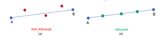
The rotor speed versus frequency plots are generated from the .out file in HyperGraph 2D. An example is shown below with X request as Mode 1.
Example of Control options in HyperGraph 2D for Plotting the Campbell Diagram.

X Type

Subcase: 1 Campbell Summary

X Request

Mode 1

X Component

Rotor Speed

Y Type

Subcase: 1 Campbell Summary

Y Request

All Required Modes

Y Component

Frequency

Figure 5. Control Options in HyperGraph 2D
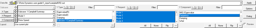
From the Plot Browser, all the required curves are chosen. Right-click Multiple Curves Math, then select Campbell Diagram.
The Campbell Diagram dialog opens.
Figure 6. Plot Campbell Diagram in HyperGraph 2D
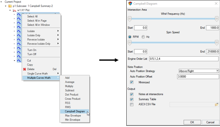
In the Campbell Diagram dialog, set the options in Figure 6 and click OK.

Figure 7. Campbell Diagram in HyperGraph 2D

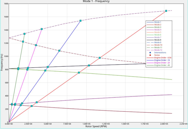
Rotor Superelements

Rotors in frequency response and complex eigenvalue solutions can be replaced using superelements.

Superelements can be attached to the grids that define the rotor in the ROTORG Bulk Data Entry. Craig-Bampton Nodal Formulation (CBN) or Guyan Reduction (GUYAN) can be specified on the METHOD field in the CMSMETH Bulk Data Entry to generate the superelements. The superelement replaces the beam elements used to model the rotor. The ASET grid points should correspond to the GRIDi points specified on the ROTORG Bulk Data Entry. The interface grid points of the superelement used to model the rotor should be exactly the same grid points defined on the ROTORG Bulk Data Entry. The General Modal Formulation (GM method) cannot be used to generate superelements for rotor dynamics.

Note: The Inertia (I66) and equivalent mass information pertaining to the Rotor superelement at the ASET connection points is printed to the .out file. This inertia information can subsequently be utilized to aid in replacing the rotor superelement with equivalent CONM2 concentrated mass elements.

Output

The rotor speed, eigenvales (real and imaginary), frequency, damping and whirl details are printed for each mode, under Campbell diagram Summary in the .out file. An example is shown below.

Subcase: 1 
                           Campbell Diagram Summary
 
 Mode #: 1 
 -------------------------------------------------------------------------------
 Step  Rotor speed   Eigenvalue  Eigenvalue     Frequency    Damping     Whirl 
           (RPM)         (Re)        (Im)          (Hz)
 -------------------------------------------------------------------------------
   1    0.000E+00  -1.92148E-01 -3.81017E+02    6.064E+01    1.009E-03  LINEAR
   2    2.000E+02  -1.92108E-01 -3.81011E+02    6.064E+01    1.008E-03  BACKWARD
   3    4.000E+02  -1.91987E-01  3.80993E+02    6.064E+01    1.008E-03  BACKWARD
   4    6.000E+02  -1.91788E-01 -3.80964E+02    6.063E+01    1.007E-03  BACKWARD
   5    8.000E+02  -1.91513E-01  3.80924E+02    6.063E+01    1.006E-03  BACKWARD
   6    1.000E+03  -1.91163E-01  3.80873E+02    6.062E+01    1.004E-03  BACKWARD
   7    1.200E+03  -1.90742E-01  3.80810E+02    6.061E+01    1.002E-03  BACKWARD

 Mode #: 2 
 -------------------------------------------------------------------------------
 Step  Rotor speed   Eigenvalue  Eigenvalue     Frequency    Damping     Whirl 
           (RPM)         (Re)        (Im)          (Hz)
 -------------------------------------------------------------------------------
   1    0.000E+00  -1.92148E-01  3.81017E+02    6.064E+01    1.009E-03  LINEAR
   2    2.000E+02  -1.92108E-01  3.81011E+02    6.064E+01    1.008E-03  BACKWARD
   3    4.000E+02  -1.91987E-01 -3.80993E+02    6.064E+01    1.008E-03  BACKWARD
   4    6.000E+02  -1.91788E-01  3.80964E+02    6.063E+01    1.007E-03  BACKWARD
   5    8.000E+02  -1.91513E-01 -3.80924E+02    6.063E+01    1.006E-03  BACKWARD
   6    1.000E+03  -1.91163E-01 -3.80873E+02    6.062E+01    1.004E-03  BACKWARD
   7    1.200E+03  -1.90742E-01 -3.80810E+02    6.061E+01    1.002E-03  BACKWARD

Note:

In rare cases, when the job is run in different machines, a given model might show flip in the sign of imaginary eigenvalues between a pair of modes. This is due to numerical differences while ordering the modes.
As the roots are complex conjugates, if the sign changes for a particular step (that is, rotor speed) in a mode, then the same step will have opposite sign in a consecutive mode.