Electrostatic Analysis

An electrostatic analysis involves the calculation of electric potential in dielectric structures subjected to electrical loads.

The basic finite element equation to be solved for structures experiencing electrical loads can be expressed as:

K_{C} φ = f

Where,

$K_{C}$: Electrical permittance matrix
$φ$: Electric potential
$f$: Electric charge

This equilibrium equation of electric charge is solved for the unknown electric potential.

Electrostatic Analysis in OptiStruct

A standalone electrostatic analysis subcase in OptiStruct can be defined using ANALYSIS=ESTAT. Two types of loading can be defined in this analysis, namely charge or enforced potential which are time independent in nature. ESTAT is used for finding electric potential distribution in dielectric material, and evaluating electrostatic force on the structure, which can be used as external loading in structural analysis.

Example:

SUBCASE 1
   ANALYSIS ESTAT
   SPC = 1
   LOAD = 2
   TEMP(MAT) = 4

Input

A summary of the relevant input file entries in an electrostatic analysis.

The relevant Subcase Information Entries are:

Table 1. Subcase Information Entries
Entry	Purpose
ANALYSIS = ESTAT	Defines an electrostatic analysis subcase

The relevant Bulk Data Entries are:

Table 2. Bulk Data Entries
Entry	Purpose
SPC, SPCD	Potential
CHARGE	Nodal charge
CHGAREA	Area Charge Density
CHGVOL	Volume Charge Density
MAT1PT	Isotropic Permittivity Material
MAT2PT	Anisotropic Permittivity Material
MATT1PT, MATT2PT	Temperature Dependent Material
PGAPES	Electrical permittance properties for gap elements
PCONTES	Contact Permittance Coefficient (CPC) for CONTACT element

Note: In MAT1PT and MAT2PT, relative permittivity and absolute permittivity can be defined. When relative permittivity is defined, vacuum permittivity must be provided by PARAM, VAPMTV. Make sure the value of the vacuum permittivity is aligned with the physical quantity used in the model.

Analogy

The following table summarizes the analogy of some electrical analysis entries with the existing thermal/structural analysis.

Table 3. Analogy for Electrical Analysis
Type	Electrostatic Analysis	Electrical Conduction Analysis	Thermal Analysis	Structural Analysis
Result output	Electrical potential	Electrical potential	Temperature	Displacement
	Electrical field	Electrical field	Temperature Gradient	Strain
	Electrical displacement	Current density	Heat flux	Stress
Loads and boundary conditions	CHARGE	CURRENT		FORCE
	CHGAREA	CDENST4	QBDY1	PLOAD4
	CHGVOL		QVOL	GRAV
	SPC (Electric potential)	SPC (Electrical potential)	SPC (Temperature)	SPC (Displacement)
	SPCD (Electrical potential)	SPCD (Electrical potential)	SPCD (Temperature)	SPCD (Displacement)
	MPC (Electric potential)	MPC (Electric potential)	MPC (Temperature)	MPC (Displacement)
Material	MAT1PT	MAT1EC	MAT4	MAT1
	MAT2PT	MAT2EC	MAT5	MAT9
	MATT1PT	MATT1EC	MATT4	MATT1
	MATT2PT	MATT2EC	MATT5	MATT9

Problem Setup

Example of an electrostatic analysis.

The following snippet of an input file gives an example of an electrostatic analysis setup:

$ *************************************************************
$ EXAMPLE TO DEMONSTRATE AN ELECTRICAL ANALYSIS SETUP
$ *************************************************************
OLOAD     = 11 
VOLTAGE   = 11    
GPCHARGE = 11    
ESTATFORCE(COMP,ESET=10) = 20
 
  
SUBCASE        2
  LABEL ELECTROSTATICS
  ANALYSIS ESTAT
  LOAD   =   3
  SPC     =  10
  

BEGIN BULK
$ vacuum permittivity
PARAM,VAPMTV,8.8541878128130E-12  
...

Example

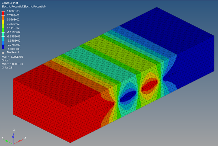
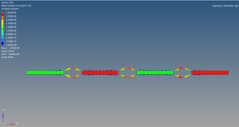
This example demonstrates the modeling of electrostatic force in an electrode system.

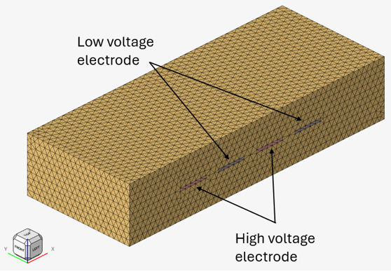
The model consists of 4 electrodes, 2 of them are with high voltage (1000V), and the other 2 are with low voltage (-1000V). Air domain surrounding the 4 electrodes are also included in the model.

Non-zero SPC is applied to the grids on electrode.

Figure 2. Electric Potential Distribution on System

Figure 3. Electrostatic Force on Grids of Electrodes

Output

Supported output requests for electrostatic analysis.

Currently, results are available in .h3d format in a separate *_estat.h3d file. Electrostatic force can be output in ASCII format.

Table 4. Supported Output Requests for Electrostatic Analysis
Result	Purpose	Details
VOLTAGE	Voltage	Available by default
ELECFLUX	Electric Displacement
ELECFIELD	Electric field	Available by default
GPCHARGE	Grid Point Charge
OLOAD	Applied nodal charge
SPCCHARGE	Reaction Charge
MPCFORCE	MPC Charge (Free Charge inducted on outer surface of a conductor)
ESTATFORCE	Electrostatic force

A charge balance summary table is available in the .out file for electrostatic analysis. This is similar to the SPCFORCE output table and consists of total applied charge and SPC charge.