Complex Eigenvalue Analysis

Real eigenvalue analysis is used to compute the normal modes of a structure. Complex eigenvalue analysis computes the complex modes of the structure.

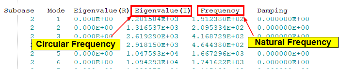
The complex modes contain the imaginary part, which represents the cyclic frequency, and the real part which represents the damping of the mode.

If the real part is negative, then the mode is said to be stable. If the real part is positive, then the mode is unstable. Complex eigenvalue analysis is usually used to determine the stability of a structure when unsymmetric matrices are presented due to special physical behavior. It is also used to determine the modes of a damped structure.

The complex eigenvalue analysis is formulated in the following manner:(1)

(λ^{2} M + λ C + ((1 + i g) K + i C_{G E} + α_{f} K_{f})) A = 0

Where,

$K$: Stiffness matrix of the structure
$M$: Mass matrix
$C_{G E}$: Element structural damping matrix
$C$: Viscous damping matrix
$g$: Global structural damping coefficient
$K_{f}$: Extra stiffness matrix defined by direct matrix input
$α_{f}$: Coefficient of extra stiffness matrix

The solution of the complex eigenvalue problem yields complex eigenvalue, $λ = α + i β$ , and complex mode shape, $A$ . Complex modes with positive real parts are considered unstable modes. Unstable modes are often generated in pairs.

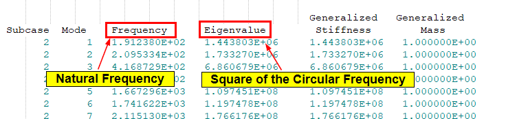
The circular frequency,

ω

is the same as

β

:(2)

ω = β = 2 π f

Where, $f$ is the natural frequency.

In the .out file, for the complex modes, the complex eigenvalue is the same as the circular frequency, while the frequency printed is the natural frequency.

For the real modes, the eigenvalue printed is the square of the circular frequency.

The damping coefficient is also computed from:(3)

c = - \frac{2 α}{| β |}

This corresponds to the real part of a complex eigenvalue; modes with negative damping coefficients have positive real parts and are unstable modes.

Direct Complex Eigenvalue Analysis

The extraction of complex modes can be accomplished directly from the above formulation. It is important to note that this is computationally expensive.

To run a direct complex eigenvalue analysis, the EIGC Bulk Data Entry needs to be specified, as it defines the number of complex modes to be extracted. The EIGC card is referenced by a CMETHOD statement in the same SUBCASE definition.

Modal Complex Eigenvalue Analysis

The extraction of complex modes directly from the above formulation is usually quite computationally expensive, especially if the problem size is not small. Instead, a modal method is used to solve the complex eigenvalue problem. First, the real modes are calculated via a normal modes analysis. Then, a complex eigenvalue problem is formed on the projected subspace spanned by the real modes and thus much smaller than the real space. Finally, the complex modes extraction of the reduced problem follows the well-known Hessenberg reduction method.

To run a model complex eigenvalue analysis, both the EIGRL and EIGC Bulk Data Entries need to be specified. They define the number of the real modes and the number of complex modes to be extracted, respectively. The EIGRL card should be referenced by a METHOD statement in a SUBCASE definition. The EIGC card is referenced by a CMETHOD statement in the same SUBCASE definition.

Output

Complex eigenvalues and frequencies are printed in the .out file for both Direct and Modal Complex Eigenvalue Analysis. For Complex Eigenvalue Analysis involving rotor dynamics, the sorting and listing of modes in the .out file is based on the magnitude of the eigenvalues. For complex eigenvalue runs without rotor dynamics, the sorting is based on the imaginary part of the eigenvalues.

For Complex Eigenvalue Analysis involving rotor dynamics, complex conjugate mode pairs (if any) are printed in the .out file. This is not the case for Complex Eigenvalue Analysis without rotor dynamics.

Note: As an exception, complex conjugate mode pairs are not printed to the .out file for rotor dynamics using Complex Eigenvalue Analysis if it is a SYNC Analysis without damping and only contains a single rotor in the input file.

Additional output for Acoustic (coupled fluid structure) Complex Eigenvalue Analysis can also be exported to a .cmode.csv file file. For more information, refer to the PARAM, FCACSV Bulk Data Entry.

Usage

The complex eigenvalue solution usually involves an unsymmetrical matrix which represents the source of the physical instability (like friction). The following applications are currently available with complex eigenvalue analysis:

Brake Squeal Analysis

To capture this instability, a nonlinear static analysis (small displacement) subcase should be setup and the model state can be carried over to the modal complex eigenvalue analysis subcase using STATSUB(BRAKE). If STATSUB(BRAKE) is present, then OptiStruct transfers the various parameters associated with the model state (stress, geometric stiffness, friction, and so on) at the end of the referenced NLSTAT subcase and performs the modal complex eigenvalue analysis. This workflow is typical in brake squeal analysis applications.

Brake Squeal with External Friction Matrix

In some cases, instead of using STATSUB(BRAKE) you may choose to import an external matrix to represent the friction state of the model prior to a Modal Complex Eigenvalue solution. The external matrix should be provided as a DMIG Bulk Data Entry, and then referenced by a K2PP statement in the SUBCASE definition. You can define a specific coefficient for the external matrix by PARAM, FRIC. Otherwise, the default value of the coefficient is 1.0.

Rotor Dynamics

Complex eigenvalue analysis is also utilized to model the gyroscopic effect of rotating systems via rotor dynamics.