This newly developed OptiStruct Explicit solution type
(ANALSIS=NLEXPL) has been developed solely in
OptiStruct, in the same way as the OptiStruct implicit solution. The input data (elements, material,
property, loading, and so on) for explicit solution is the same as implicit solution and the
output data structure is also the same as implicit solution.
This solution sequence performs Nonlinear Explicit Finite Element Analysis. The
predominant difference between Nonlinear Explicit Finite Element Analysis and
Nonlinear Implicit Transient Analysis is the time integration scheme. In Nonlinear
Explicit Finite Element Analysis, time step is usually smaller, and no matrix
assembly and inversion is required in explicit analysis as compared to implicit
approaches. The OptiStruct Nonlinear Explicit solution
sequence generally supports all major nonlinear features, for instance, Geometric
Large Displacement Nonlinearity, Material Nonlinearity, and Contact. Subcase
continuation, is currently not supported.
SMP, MPI (DDM), and hybrid parallelization are supported for OptiStruct Nonlinear Explicit Analysis. Single precision and
double precision executables are both supported for OptiStruct Explicit Analysis.
Nonlinearity Sources
Geometric Nonlinearity
In analyses involving geometric nonlinearity, changes in geometry as the structure
deforms are considered in formulating the constitutive and equilibrium equations.
Many engineering applications require the use of large deformation analysis based on
geometric nonlinearity. Applications such as metal forming, tire analysis, and
medical device analysis.
Material Nonlinearity
Material nonlinearity involves the nonlinear behavior of a material based on current
deformation, deformation history, rate of deformation, temperature, pressure, and so
on.
Constraint and Contact Nonlinearity
Constraint nonlinearity in a system can occur if kinematic constraints are present in
the model. The kinematic degrees-of-freedom of a model can be constrained by
imposing restrictions on its movement. For RBE2,
RBE3, MPC, and TIE
contact, constraints are enforced in a kinematic way by default.
RBE3, MPC and TIE
switch to penalty approach if over-constraints are detected.
In the case of contact, the constraint condition is enforced by penalty method.
Auto-contact is available by setting the TYPE field to
AUTO on the CONTACT Bulk Data Entry.
Follower Load
Applied loads can depend upon the deformation of the structure when large
deformations are involved. Geometrically, the applied loads (Forces or Pressure) can
deviate from their initial direction based on how the model deforms at the location
of application of load. In OptiStruct, if the applied
load is treated as follower load, the orientation and/or the integrated magnitude of
the load will be updated with changing geometry throughout the analysis.
Applied loads can be indicated as follower loads using the FLLWER
Bulk and Subcase Entries, and/or with the PARAM,FLLWER entry.
Note: Follower loading is currently supported for loads specified via
DLOAD/TLOAD#, for all pressure loads,
FORCE1, FORCE2,
MOMENT1 and MOMENT2.
Explicit Finite Element Analysis Method
In explicit finite element method, the time-discretized equation is solved using
explicit time integration method. The explicit time integration method is based on the
central difference scheme.
Central Difference Method
In the Central Difference method, the equilibrium equation takes the following
form:
Where,
Lumped mass matrix
, , , and
Are the external force, damping force, contact force, hourglass force
and element internal force vectors, respectively.
Computed directly from the equilibrium equation.
From velocity and displacement vectors can be updated
as:
Where,
Current time
Next time
The following time increments are defined:
Then,
Critical Time Step
Unlike implicit nonlinear transient analysis, explicit time integration scheme is
conditionally stable.
The explicit solution marches forward in time. The time-step at each time increment
is calculated automatically by default (elemental time step is the default), and can
be switched between elemental and nodal time step using the TYPE
field of the TSTEPE Bulk Data Entry. The DTMIN
field on TSTEPE Bulk Data Entry can be used to specify a minimum
allowed nodal time increment. The top ten smallest critical timesteps
(elemental/nodal) are printed in the .out file by default for
Explicit Dynamic Analysis. This can be controlled using PARAM,
CRTELEM.
Elemental Time Step
This is the default time step control type for Nonlinear Explicit Analysis. The
TYPE field on TSTEPE entry is set to
ELEM by default.
Solid Elements
The time step size should satisfy:
Where, denotes the maximum natural frequency of
the system.
For solid elements, a critical time step size is
computed from:
Where,
Adiabatic sound speed
A function of the bulk viscosity coefficients and
Where,
and
Bulk viscosity coefficients, are dimensionless constants
with default values of 1.5 and 0.06, respectively.
Element characteristic length.
8 node hexahedron
10 node tetrahedron
6 node pentahedron
4 node tetrahedron
Where,
Symmetric gradient of shape function
Volume of the hexahedron element
Maximum area among all the six faces of the hexahedron
element
Shell Elements
For shell elements, the time step size is determined
by:
Where, is the speed of sounds, which is
calculated as:
Where,
Young's modulus
Density
Poisson's ratio
Characteristic length, which is calculated as for
quadrilateral elements:
Where,
Area
Lengths of the sides of the triangle elements:
Where,
Area
Lengths of the sides of the element
Spring Elements
For spring elements (lumped spring-mass system) there is
no wave propagation speed to calculate the critical time-step
size.
The eigenvalue problem for the free-vibration of a spring
with nodal masses, and , and stiffness, , is:
Since the determinant of the characteristic
equation should equal zero, the maximum eigenvalue can be solved
for:
Where, .
Based on the critical time-step
of a truss element:
and , you can
write:
Approximating the spring masses by using half
of the actual modal mass, you obtain:
Therefore, in terms of the nodal mass, the
critical time step size can be written:
This does not take damping into consideration.
If damping is defined, the time step is scaled by:
Where,
and
Nodal masses.
Stiffness in the corresponding degree of freedom.
Damping coefficient (for CBUSH elements,
it is defined via the Bi fields of the
PBUSH Bulk Data Entry).
Nodal Time Step
The time step control can be switched from the default elemental time step to nodal
time step by setting the TYPE field on TSTEPE
Bulk Entry to NODA.
The nodal time step is calculated as:
Where,
Nodal mass
Nodal stiffness (which is calculated from the elemental stiffness)
Nodal stiffness is calculated as:
For each element, the critical time step, is calculated first, and each node is assumed to
have the same time step, , then for each node, you can estimate the nodal
stiffness from this equation.
Where,
The i-th node of the element
Nodal mass of the i-th node
Nodal stiffness of the i-th node of this element
Therefore, the nodal stiffness of the i-th node is:
The final nodal stiffness is:
Using , the nodal critical time step can be calculated.
Mass Scaling
Elemental Mass Scaling
The elemental mass can be scaled to increase , if the scaled elemental critical time
step (scaled by DTFAC), falls below
DTMIN. This is possible since the elemental time
step equation contains the speed of sound term (), which is dependent on material density
().
Nodal Mass Scaling
The nodal mass can be scaled to increase , if the scaled nodal critical time step
(scaled by DTFAC), falls below
DTMIN.
Mass Scaling Controls
Mass scaling in a succeeding Explicit Dynamic
Analysis subcase can be controlled through the MSCALE Subcase Information Entry. When
MSCALE is not defined, the mass scaling will
continue from the preceding Explicit Dynamic Analysis subcase.
Hourglass Control
Hourglass control can be activated using PARAM,HOURGLS or
HOURGLS entries. These entries also provide access to adjust
hourglass control parameters (HGTYP and HGFAC).
If the HOURGLS entry is input, then it should be chosen via
HGID field on the corresponding Property entry to be
activated. HOURGLS entry via HGID field
overwrites the settings defined via PARAM,HOURGLS.
For Solid Elements
For solid elements with MAT1/MATS1 material,
two types of hourglass control are provided:
Type 1 (Flanagan and Belytschko, 1981) resists undesirable hourglass modes
with viscous damping.
Type 2 (Puso, 2000), uses an enhanced assumed strain physical stabilization
to provide coarse mesh accuracy with computational efficiency. Type 2 is
chosen as the default hourglass type for
MAT1/MATS1 material for 1st order
CHEXA elements.
The implementations of Type 1 and Type 2 hourglass controls are very similar, except
that the hourglass forces are calculated in a different manner.
Note: Type 2 is more
computationally intensive; however, performs better in eliminating Hourglass
modes, when compared to Type 1. The only limitation of Type 2 is that it may
lead to an overly stiff response in bending problems with large plastic
deformation.
For MATHE entry, the default hourglass control is Type 4 (Reese,
2005). Type 2 is also available for MATHE entries.
In case of reduced integration for solid elements
(ISOPE=URI), hourglass control is turned on
by default.
Dynamic relaxation can be used to solve static or quasi-static problems using an
Explicit Dynamic Analysis, by avoiding dynamic oscillations. Compared to an implicit
analysis, it could be more efficient and robust in some cases with high
nonlinearities (for example, with many complicated contacts). Examples of typical
applications include 3-point bending simulations of phone structures and spring back
simulation in sheet metal forming.
Unlike conventional dynamic relaxation which requires at least one input, OptiStruct supports adaptive dynamic relaxation via the DYREL entry, for which no input parameters are needed. The
damping factor is automatically determined based on the system’s highest natural
frequency.
Material Failure Criterion
Material failure criterion can be defined using the MATF
Bulk Data Entry or the MATS1 Bulk Data Entry (for damage
initiation/evolution criteria only). Failure of materials is strongly influenced by
the loading conditions and thus, the stress state. Hence, several criteria available
refer to the notions of stress triaxiality and optionally to the Lode parameter to
describe the loading conditions (uniaxial tension, pure shear, plane strain
etc).
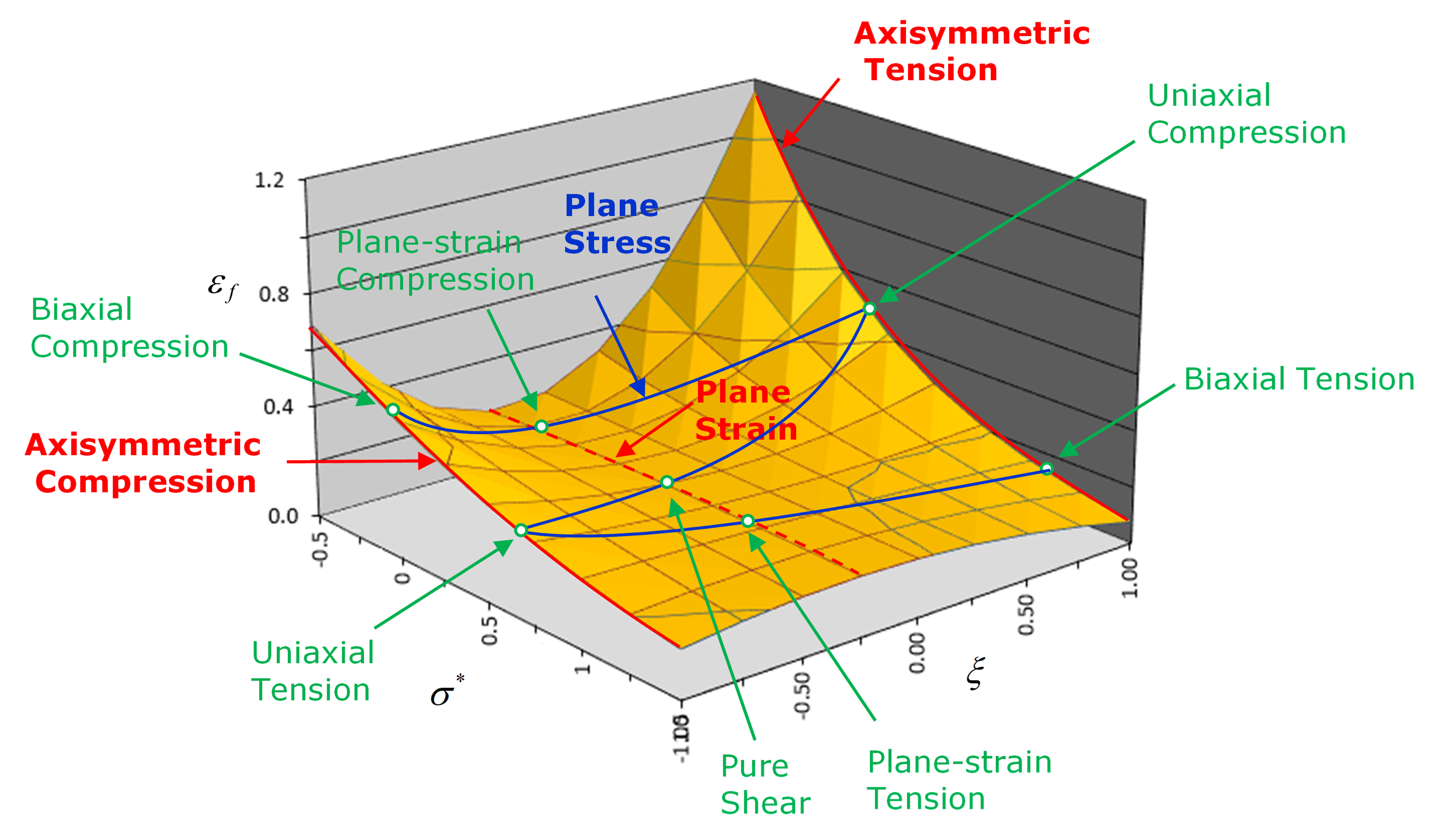
To describe a failure criterion based on plasticity and stress states, the value
stress triaxiality, , and the lode parameter, , are needed. For shells only, stress triaxiality is needed.
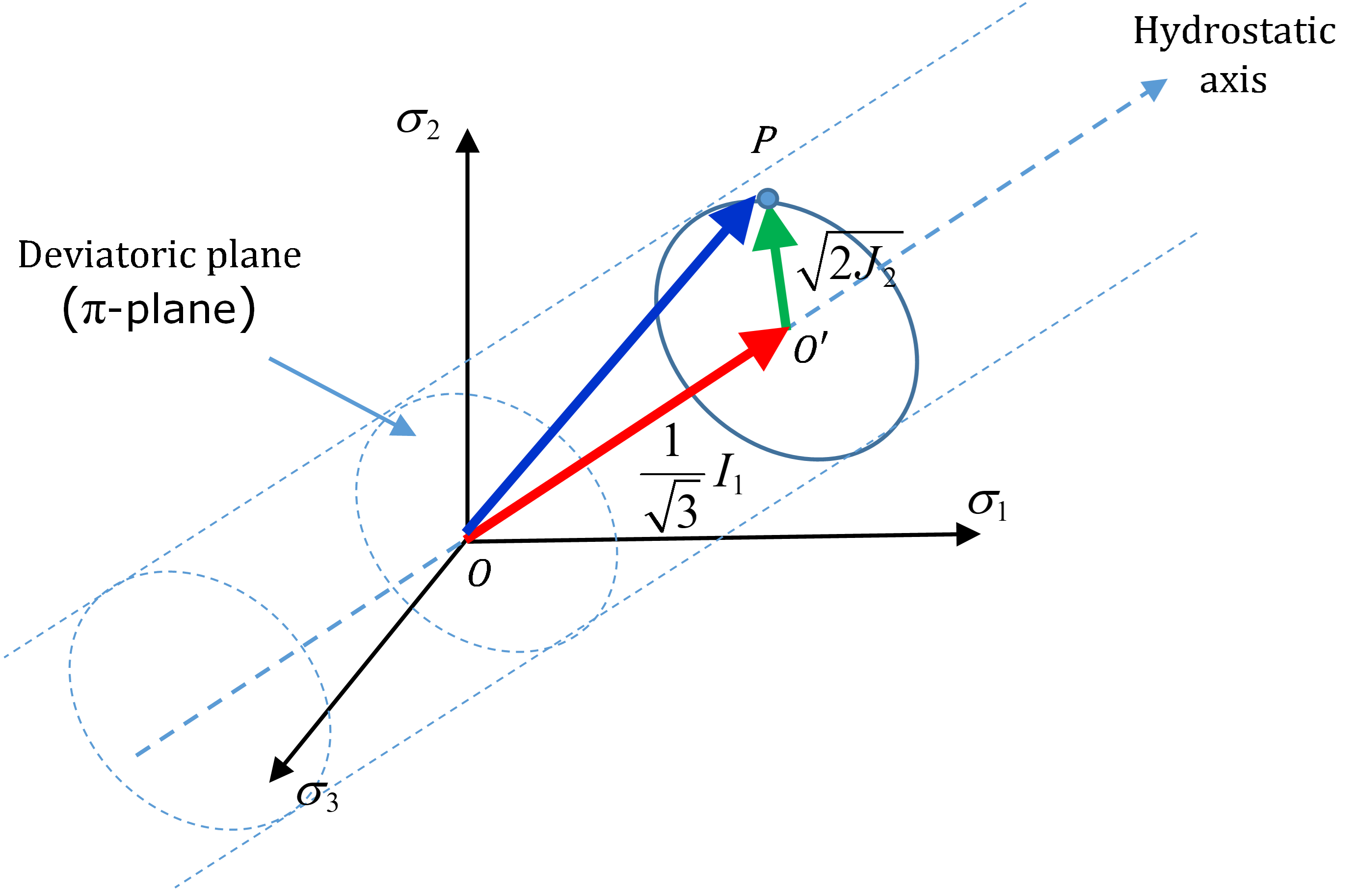
Stress Triaxiality
Stress triaxiality () is used to differentiate between compressive and tensile loadings and depends on
the trace of the stress tensor. It can determine the position of the stress state on
the hydrostatic axis shown in Figure 1.Figure 1. Description of the stress state on hydrostatic axis and
deviatoric plane It is computed as follows:
Where is the equivalent von Mises stress.
The values of stress triaxiality vary from to for solids (in practice bounded to -1 and 1) and
-2/3 to 2/3 for shells.
Table 1. Stress triaxiality values for some common stress
states
Loading condition
Solids
Shells
Confined compression
-1
Biaxial compression
-2/3
-2/3
Uniaxial compression
-1/3
-1/3
Pure shear
0.0
0.0
Uniaxial tension
1/3
1/3
Plane strain
0.5751
0.5751
Biaxial tension
2/3
2/3
Confined tension
1
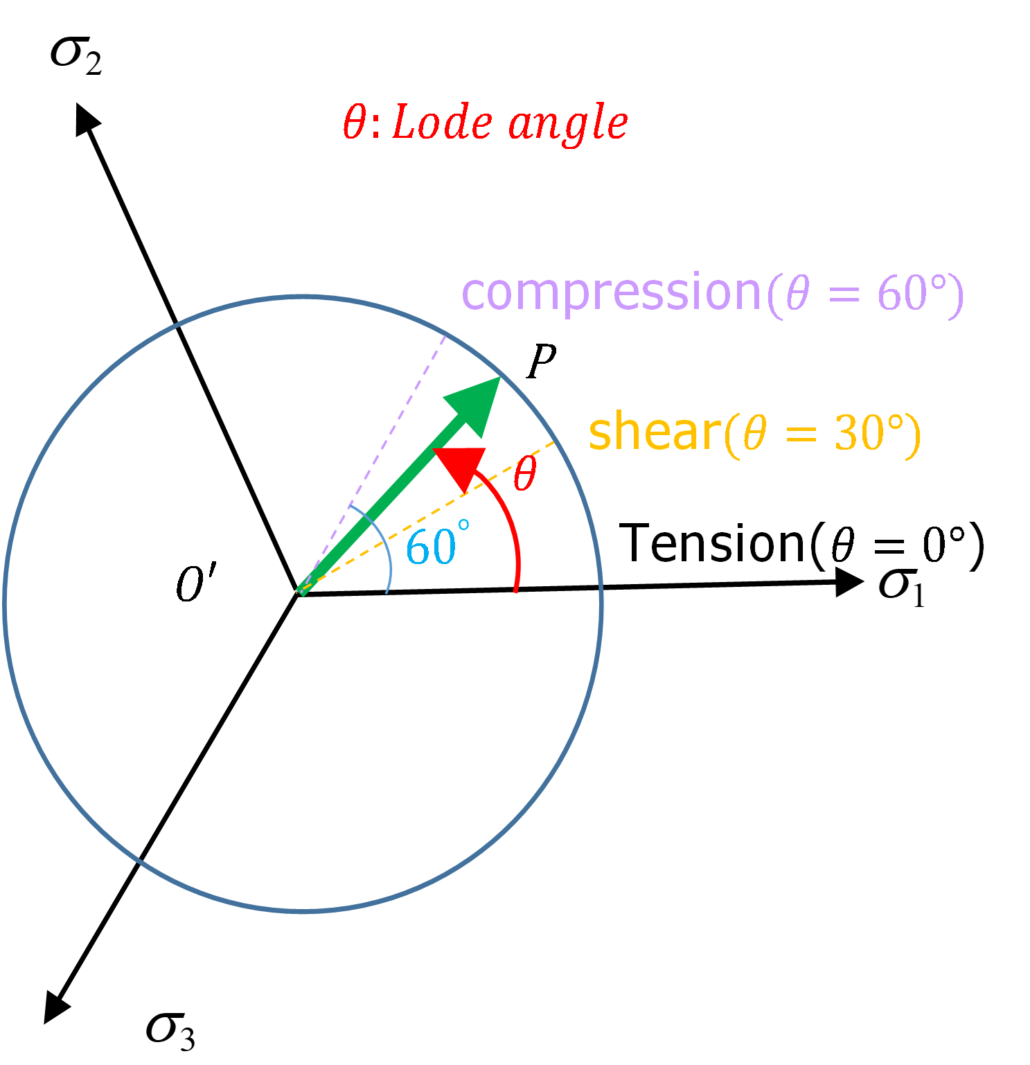
Lode Angle
To describe 3D loading conditions, another important quantity is the lode angle
() given by:
Where is the third deviatoric invariant.
The lode angle determines the position of the stress state in the deviatoric section.
Its value is between 0 (for tension) and (for compression).Figure 2. Stress state position on the deviatoric plane depending on
the lode angle value Shear and plane strain condition takes a lode angle value of .
Under plane stress hypothesis (for shell elements), the lode angle and the stress
triaxiality are linked and thus one for them can be used to recover the
other:
As it is much easier to deal with normalized value instead of radians, the lode angle
is usually switched by the Lode parameter denoted , given by:
The lode parameter's values are:
-1.0 in compression
In pure shear or plane strain
In tension
Supported Failure Criteria
Currently, four failure criteria are supported for Explicit Dynamic Analysis namely,
BIQUAD, TSTRN, tabulated failure criteria and INIEVO.
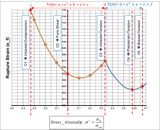
BIQUAD
The BIQUAD criterion is a stress triaxiality based failure criterion
mostly used for ductile metals. Its double quadratic curve shape
describes the evolution of plastic strain, , at failure with respect to stress
triaxiality, , as shown in the below image.Figure 3. Failure plastic strain evolution with stress
triaxiality for BIQUAD criterion It then requires five parameters called c1, c2, c3, c4 and c5
respectively corresponding to V1,
V2, V3, V4
and V5 value in the MATF Bulk Data
Entry. These five values correspond to plastic strain at failure for
five different stress states:
Uniaxial compression
Pure shear
Uniaxial tension
Plane strain
Biaxial tension
Note: The parabolic curve computation at high stress triaxiality is
made so that c4 is always the minimum value.
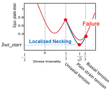
For shell
elements, strain localization and necking occurring at high strain rate
might not be correctly detected as the thickness variation is purely
numerical. Thus, failure can be delayed in comparison to an equivalent
sized solid element. To avoid that, an additional curve (see the blue
curve in the below figure) can be defined for shells using INST
parameter (V6), replacing c4 in the high stress
triaxiality parabolic curve computation.Figure 4. Additional failure quadratic curve (in blue) at
high stress triaxiality for shells If enough experimental data is unavailable to identify all the c1,
c2, c3, c4 and c5 parameters, a material selector input is also
available for BIQUAD criterion. Depending on the keyword MATER value
chosen in the list presented above, the c1, c2, c4 and c5 parameters
will be automatically computed with respect to c3 value, as shown
below.
The value c3 is then the only expected parameter when
using material input for BIQUAD criterion. However if no c3 value is
specified, a default value of c3 will automatically be set.
Table 2. Automatic parameters settings for MATER
keyword
Keyword
c3 (Default)
r1
r2
r4
r5
MILD
0.60
3.5
1.6
0.6
1.5
HSS
0.50
4.3
1.4
0.6
1.6
UHSS
0.12
5.2
3.1
0.8
3.5
AA5182
0.30
5.0
1.0
0.4
0.8
AA6082
0.17
7.8
3.5
0.6
2.8
PA6GF30
0.10
3.6
0.6
0.5
0.6
PP T40
0.11
10.0
2.7
0.6
0.7
For each timestep, the plastic strain at failure, , is estimated according to the stress
triaxiality and the parabolic curves. This allows increases to the
damage variable accounting for the stress state history:
TSTRN
The TSTRN failure criterion is a strain based damage model and is
supposed to be fully coupled (DAMAGE keyword
activated and ). However, you have the freedom to use
it as a failure criterion or a pure output damage variable. It considers
a linear evolution of the damage variable between two starting and
ending strain values, in tensile loading conditions ():
A couple of values and are then needed in the card.
V1 and V2 values corresponds
to starting and ending von Mises equivalent strain. The von Mises
equivalent strain is computed as follows:
Where is the deviatoric strain tensor.
If
V3 and V4 values are
specified, they correspond to starting and ending major principal
strain.
Note:V3 and
V4 values are always prioritized when
both V1/V2 and
V3/V4 pairs are
specified.
Tabulated failure criteria
The TAB failure criterion is used to give as much freedom as possible to
describe a plastic strain based tabulated criterion. The
TABLEMD entry defined by EPS_TID describes the
map showing the evolution of plastic strain at failure, , with respect to stress triaxiality and,
optionally for solid elements, with lode parameter, , as shown in Figure 5.Figure 5. Tabulated failure criterion map showing the
evolution of plastic strain at failure with respect to stress
triaxiality and lode parameter For solid elements, the entire map with all possible couple of
values, , is considered. However, for shells
stress triaxiality and lode parameter are linked due to plane stress
conditions. Hence, only the plane stress (blue line in Figure 5) is considered.
The V1 value is a scale factor
that allows you to quickly increase or decrease in entire
map.
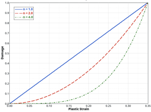
The damage variable evolution is given by a specific
formula using the parameter in defined in V2 value:
Thus, including its own current value, the damage
variable evolution is taking into account the stress state history
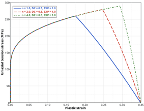
but also the damage history. The exponent allows to indirectly change the
shape of the damage evolution with respect to plastic strain as
presented in Figure 6. The increase of the exponent parameter tends to delay
the stress softening effect as shown.Figure 6. Effect of n parameter on the damage versus
plastic strain evolution (left picture) and effect of n
parameter on a single element uniaxial tension behavior
(right picture)
You can use the TAB criterion defining only
the first line of parameters (EPS_TID,
V1 and V2). In this case,
like any other criterion available, you can activate the element
deletion using DAMAGE, chose the beginning of
stress softening with the constant value for critical damage
DC and the shape of the stress softening
using EXP.
Another approach of stress
softening approach with TAB criterion is called
the necking-controlled approach.
To use this new
approach, the two first parameters of the second line
INST_TID and V6 must be
defined. INST_TID defines the ID of a
TABLEMD entry defining a map showing the
evolution of the plastic strain value (denoted ) for which necking instability and
thus strain localization starts, with respect to stress triaxiality
and, optionally, lode parameter. It is an instability limit curve or
map mostly defined at high stress triaxiality as the one described
above for BIQUAD criterion in Figure 3 and is supposed to be lower than the failure
curve/map to have an effect. It can be used with solids or
shells.
This INST second map allows to compute the evolution
of a new variable called necking-triggering variable
and denoted . Its evolution is very similar to
the damage variable one:
Once this variable reaches the value 1, a
stress softening is triggered (defined by Comment 12 in the MATF Bulk Data
Entry). However, instead of using the constant value, , in the MATF
entry, the parameter, , becomes an integration point. Thus can be very different from one
element to another depending on the history of the element stress
state.
Thus, when INST_TID is used, the value corresponds to the value taken
by the damage variable at the exact moment when reaches or overtakes the value 1. In
other words, is the value when the necking criterion is
reached the first time. Then, remains untouched until the end of
the simulation.
Unlike the parameter, the exponent
(EXP) is a constant parameter over all
elements.
This necking-controlled approach can offer a higher
predictivity for a large range of stress state but needs to define
an instability map especially at high stress triaxiality when
necking is more likely to happen.
Finally, parameters
V7 and V8 values are
stress triaxiality boundaries for element size scaling defined
below. If this pair of values are defined, the size scaling only
occurs when:
Damage initiation and evolution (INIEVO)
INIEVO failure criterion is very specific and provides the ability to
define a failure approach based on the use of a DMGINI Bulk Data Entry and, optionally a DMGEVO Bulk Data Entry.
For the
DMGINI Bulk Data Entry, only DUCTILE
criterion is available. For the DMGEVO Bulk Data
Entry, only DISP and ENERGY evolution are available.
This
criterion can be defined using two methods:
The DAMAGE continuation line in the MATS1 Bulk Data Entry.
This method is supported both for Implicit and Explicit
Dynamic Analysis.
CRI=INIEVO in the MATF Bulk Data Entry. This method is
supported only for Explicit Dynamic Analysis.
Note: For INIEVO, strain rate dependency and element size
dependency are not available.
Problem Setup
Input
Activation:
A Nonlinear Explicit Subcase can be identified via
ANALYSIS=NLEXPL. The
TTERM Subcase Entry is mandatory to define the
termination time. Additionally, a TSTEPE Subcase Entry
which points to the corresponding TSTEPE Bulk Data Entry
is also available for Nonlinear Explicit Analysis. If
TSTEPE Subcase Entry is not defined, then
ANALYSIS=NLEXPL is mandatory in
conjunction with TTERM. Otherwise,
TTERM and TSTEPE together is
sufficient to identify the Explicit Nonlinear subcase. Nonlinear Explicit
Analysis is always large displacement analysis.
Initial Conditions:
The initial conditions can be defined using
IC Subcase Entry and in conjunction with the
TIC Bulk Data Entry. The initial temperature field
can be defined using TEMP(INIT) which uses the referenced
temperature field to lookup the TABLEMD entry for the
initial material data on the corresponding MATS1
entry.
Loading:
Loads can be defined using LOAD,
DLOAD, and TLOAD# Bulk Data
Entries which should be referenced in the subcase using
DLOAD Subcase Entry. For reference via
LOAD Subcase Entry or TLOAD# Bulk
Entry, only the FORCE, FORCE1,
FORCE2, MOMENT,
MOMENT1, MOMENT2,
PLOAD2, PLOAD4,
GRAV, ACCEL2, and
SPCD entries are supported for loading.
Boundary Conditions:
Boundary Conditions can be applied via
SPC Bulk Data which are referenced by a corresponding
SPC subcase entry. Multi-Point Constraints
(MPCs) are also supported.
Subcase Continuation:
Implicit-explicit chaining is supported with the
explicit dynamic subcase. The explicit dynamic subcase can be chained with
any nonlinear implicit analysis subcase via CNTNLSUB = YES/SID Subcase Information
Entry.
4-noded CTETRA, 10-noded
CTETRA, 8-noded CHEXA, and
6-noded CPENTA elements are supported.
Shell Elements
CTRIA3 and CQUAD4 are
supported.
One-dimensional Elements
CBUSH, CBEAM, and
CBAR elements are supported.
Currently, only Belytschko-Schwer Beam formulation is supported for
CBAR/CBEAM 1D elements in
Explicit Analysis.
Mass Elements
CONM2 is supported.
Note:
Offset, on elements or property for Shell elements is supported for
Explicit Analysis.
In case of CBUSH elements, Mi
fields in PBUSH definition will be used for mass
and inertia calculations. Refer to PBUSH
in the Reference Guide for more details.
For CBEAM, CBAR elements,
The continuation lines on
PBEAM/PBAR are not
supported with Explicit Analysis.
Pin flags (PA and PB)
are supported with Explicit Analysis.
Supported
Materials:
The following materials are currently supported for
Explicit Analysis:
MAT1, MAT2,
MAT8, MATS1,
MATHE, and MATVE materials are
supported. The MATVE entry should be defined under
MATHE entry.
Linear Materials
Isotropic Materials
MAT1
Anisotropic Materials
MAT2, MAT9
Orthotropic Materials
MAT8, MAT9OR
Nonlinear Materials
Elasto-plasticity (MATS1)
Johnson-Cook
Crushable Foam
Cowper-Symonds
Johnson-Holmquist
Honeycomb (MATHC)
Hyper-elasticity (MATHE)
MOONEY
MOOR
RPOLY
NEOH
YEOH
ABOYCE
OGDEN
FOAM
MARLOW
Visco-elasticity (MATVE)
Prony
BBOYCE (Bergstrom Boyce)
Cohesive Zone Modeling (CZM)
MCOHED (Traction-Opening)
MATS1 (Cohesive Continuum)
Failure Models:
Failure (MATF)
BIQUAD
TSTRN
TAB
PLAS
JOHNSON
Damage Initiation and Evolution
MATS1 (via DAMAGE continuation
line – DMGINI and DMGEVO)
MATF (INIEVO criterion –
DMGINI and DMGEVO)
Brittle Damage
MATBRT
MATF (RANKINE)
Integration Schemes:
For explicit analysis, the element integration scheme can
be changed using the ISOPE field on the
PSOLID, PLSOLID,
PSHELL, PCOMP,
PCOMPG, PCOMPP entries, or via
PARAM,EXPISOP. The settings on the
ISOPE field will overwrite the settings on
PARAM,EXPISOP.
The typical output entries (DISPLACEMENT,
VELOCITY, and ACCELERATION) can be used to
request corresponding output for Nonlinear Explicit Analysis. The
NLOUT Subcase and Bulk Data Entries can be used to request
intermediate results, only with NINT parameter support.
The NLOUT Bulk Data Entry and NLOUT Subcase Information Entry can be used to control incremental output. For
Nonlinear Explicit Analysis, only the NINT field is supported for
NLOUT. The NLADAPT entry is not supported
for Nonlinear Explicit Analysis, and no other TSTEP# entries are
supported, except TSTEPE entry.
Currently, only Hyper3D (_expl.h3d) and HyperGraph presentation format
(_expl.mvw) files are supported. Nonlinear Explicit
Analysis results are not output to the regular .h3d and
.mvw files, but instead are output to
_expl.h3d and _expl.mvw files,
respectively.
_expl.h3d
Contours for Displacement, Rotation, Velocity, Acceleration, Strain,
Strain rate (in case of rate dependent plasticity), Stress, Plastic
Strain, CBUSH element force, Composite stress,
Composite Strain and Composite failure index are output. Additionally,
in an _expl.h3d file, the initial and current nodal
mass of the model is available by default in HyperView. 8
When a monitor volume is defined via the MONVOL Bulk Data Entry, the following output results are available by
default. Pressure, Temperature, Volume, Area, Mass, Internal Energy,
Mass flow rate, Vent Area and Leaked Mass.
_expl.mvw
This session file automatically loads the corresponding
_expl.h3d file and allows you to plot the
results output in the _expl.h3d file.
_s<ID>_e.expl
Curves for Internal energy, Elastic Contact energy, Plastic Contact
energy, Kinetic energy, Hourglass energy, and Plastic Dissipation energy
are output
_expl_energy.mvw
This session file automatically loads the corresponding
_s<ID>_e.expl file and allows you to plot
the various energy output.
.out
For explicit, the .out file contains Time Cycle
information (based on PARAM,NOUTCYC), Current time,
Current Time Step, Maximum Strain Energy, Element ID for which the
information is printed, Kinetic Energy, Contact Work, Total Energy,
Maximum Penetration, Node ID associated with this maximum penetration,
Maximum Normal Work, Node ID associated with this Maximum Normal Work,
Mass Change Ratio. which is the information regarding the scaled mass
change after mass scaling – this is calculated as: (current
mass-original mass)/(original mass).
_expl.cntf
An ASCII file that contains the contact
force output results on the main surface and is activated when the
OPTI format is specified in the CONTF I/O Options Entry. The output includes
Normal/Tangential Force, Magnitude and Area of contact. This output is
available for each explicit time-step.
The frequency of output in this file can be controlled using the
NINT field in the NLOUT
entry.
_TH.h5
Time history output for Explicit Dynamic analysis is available in a
_TH.h5 file HDF5 format file. In some
situations, a subset of results (for example, energy) is required to be
output at a high output frequency. But increasing output frequency in
NLOUT would affect all results, leading to
enormous file size and this may be undesired. Time history output is a
useful and effective solution for such cases.
For more details regarding supported results, refer to the THIST Bulk Data Entry.
Table 3. Explicit Dynamic Analysis Quick Summary
Nonlinear Explicit
Analysis
Subcase or I/O
Bulk Data
Comments
Activation:
Subcase Type
ANALYSIS=NLEXPL
(optional)
NA
If TSTEPE is
not specified, then
ANALYSIS=NLEXPL is
mandatory.
Nonlinear Explicit
Activation
TTERM
(mandatory)
TSTEPE
(optional)
TSTEPE (optional)
If TSTEPE is
not specified, then
ANALYSIS=NLEXPL is
mandatory.
Loads:
Nodal Loads
LOAD, DLOAD
If LOAD in subcase is
used:
FORCE,
FORCE1, FORCE2,
MOMENT, MOMENT1,
and MOMENT2.
If
DLOAD in subcase is
used:
TLOAD1 or
TLOAD2.
DLOAD can be used to combine
multiple TLOADi data.
For nodal
loads, EXCITEID on
TLOADi data can be
FORCE, FORCE1,
FORCE2, MOMENT,
MOMENT1, and
MOMENT2.
TYPE field on
TLOADi data can be set to
0 or LOAD for this case.
Surface Loads
LOAD, DLOAD
If LOAD in subcase is
used:
PLOAD2 and
PLOAD4.
If
DLOAD in subcase is
used:
TLOAD1 or
TLOAD2.
DLOAD can be used to combine
multiple TLOADi data.
For Surface
loads, EXCITEID on
TLOADi data can be
PLOAD1 and PLOAD4.
TYPE field on
TLOADi data can be set to
0 or LOAD for this
case.
Body Loads
LOAD, DLOAD
If LOAD in subcase is
used:
GRAV and
ACCEL2.
If
DLOAD in subcase is
used:
TLOAD1 or
TLOAD2.
DLOAD
can be used to combine multiple TLOADi
data.
For Body loads, EXCITEID on
TLOADi data can be
GRAV and
ACCEL2.
TYPE field on
TLOADi data can be set to
0 or LOAD for this
case.
Enforced Displacement, Velocity,
Acceleration
LOAD, DLOAD
If LOAD in subcase is used:
Enforced
displacement, velocity, or acceleration using
SPCD or SPCD.
If DLOAD in subcase is
used:
TLOAD1 or
TLOAD2.
DLOAD can be used to combine
multiple TLOADi data.
For Enforced
loading, EXCITEID on
TLOADi data can be
SPC or
SPCD.
TYPE field on
TLOADi data can be set to:
1 or DISP
For enforced displacement,
2 or VELO
For enforced velocity,
3 or ACCE
For enforced acceleration.
Follower Loading
FLLWER
FLLWER
PARAM,FLLWER
Loads can be chosen as follower
loads, similar to implicit nonlinear analysis.
Follower
loading is currently supported for loads specified via
DLOAD/TLOAD#, for
all pressure loads, FORCE1,
FORCE2, MOMENT1
and MOMENT2.
Boundary Conditions:
Single Point Constraints
SPC
SPC
Initial Conditions:
Initial Displacement
TIC
IC
Initial Velocity
TIC
IC
Time Step Control:
Basic time controls
TSTEPE
TSTEPE
TYPE field on
TSTEPE entry to choose between elemental
and nodal time step controls.
DTMIN field
can define minimum time step below which nodal/elemental
mass scaling is activated.
DTFAC
field can define scale factor for stable time increments.
Mass Elements:
Mass Elements Support
CONM2 is supported
Structural Elements:
Supported Structural
Elements
NA
One-dimensional elements: CBUSH,
CBEAM, and CBAR are supported;
Shells
CTRIA3 and
CQUAD4 elements.
Solids
4-noded CTETRA, 10-noded
CTETRA, 8-noded
CHEXA, and 6-noded
CPENTA elements.
Integration Schemes
NA
ISOPE field on PSOLID,
PLSOLID, or
PSHELL.
PARAM,EXPISOP
(parameter is only supported for solid
elements).
ISOPE field
will overwrite settings defined on
PARAM,EXPISOP.
Refer to Elements in the User
Guide for more details regarding Integration
Schemes.
Constraints:
Support for Rigids
NA
RBE2, RBE3 and
RBODY are supported.
Materials:
Supported Materials
NA
Shells: MAT1, MAT2,
MAT8 and
MATS1.
Solids: MAT1,
MATS1, MATVE,
MAT9OR, MCOHED,
and MATHE.
Auto-Contact is supported by
setting the TYPE field to
AUTO on CONTACT Bulk
Data Entry.
For TIE in
explicit:
1
Only kinematic TIE is
supported. That is, the kinematic condition is
precisely constrained instead of using the
penalty-based method.
2
Hierarchy in kinematic TIE is
not supported (that is, secondary node of a
TIE cannot be the main node in
another TIE).
3
Over-constrained TIEs are
ignored (only the first constraint for such cases,
based on the order of input in the
.fem file, is retained).
4
All such hierarchy and over constrained
TIE nodes are printed into grid
SET in the
*_badtied.fem file.
Coordinate Systems:
Supported User-defined
Coordinate Systems
NA
CORD2R, CORD1C,
CORD2C, CORD1S, and
CORD2S
Output:
ASCII Output
NA
PARAM,NOUTCYC
Only explicit time cycle summary
and corresponding information like Time steps, Energy, Maximum
Penetration, Mass Change Ratio, and so on are printed to the
.out
file.PARAM,NOUTCYC can be used to choose
the frequency of summary output in the .out
file.
Results are output only to the
_expl.h3d and
_expl.mvw files.
_expl.h3d
The displacement, rotation, velocity, acceleration,
stress, strain, strain rate (for rate dependent
plasticity problems), CBUSH
force, plastic strain composite stress, composite
strain and composite failure index results
output.
_expl.mvw
Automatically loads the corresponding
_expl.h3d file and allows you
to plot the results output in the
_expl.h3d file.
_s<ID>_e.expl
Contains curves for Internal energy, Elastic Contact
energy, Plastic Contact energy, Kinetic energy,
Hourglass energy, and Plastic Dissipation energy
output.
_expl_energy.mvw
Automatically loads the corresponding
_s<ID>_e.expl file and
allows you to plot the various energy output.
ESE output is available with COMP and OCOMP group
options, only in the .h3d
format.
THIST can be used to
generate time history output for certain results in a
_TH.h5 file.
When a monitor
volume is defined via the MONVOL Bulk
Data Entry, the following output results are available by
default – Pressure, Temperature, Volume, Area, Mass,
Internal Energy, Mass flow rate, Vent Area and Leaked
Mass.
Output Control
NLOUT, THIST
NLOUT, THIST
Only the NINT
field is supported for Explicit Analysis.
The
NLADAPT entry is not supported for
Nonlinear Explicit Analysis.
Miscellaneous:
Large Displacement
NA
NA
Explicit Nonlinear Analysis is
large displacement nonlinear analysis by default.
The
defaults can be overwritten by user-defined PARAM,HOURGLS
or HOURGLS entry (referenced by HGID
on property entry).
You can
turn on hourglass control using PARAM,HOURGLS or
HOURGLS entry (referenced by HGID
on property entry).
For solid
elements, ISOPE field on
PSOLID/PLSOLID entries can be used
to switch between integration schemes.
Hourglass
control is not applicable for CTETRA (1st and 2nd
order).
For shell
elements, ISOPE field on PSHELL entry
can be used to switch between integration schemes.
The
defaults can be overwritten by user-defined PARAM,HOURGLS
or HOURGLS entry (referenced by HGID
on property entry). Note that for
MAT1/MATS1/MATHE,
the defaults only apply in the case of 1st order CHEXA
elements. For CPENTA elements, turn ON hourglass control,
if required.
Some
materials listed here are not supported for shells (for instance,
MATHE and MATVE).
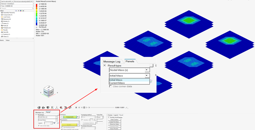
The
initial and nodal mass of an explicit model is available by default in
HyperView. Initial or current mass can be
selected from the result sub-type drop down.Figure 7. Select Initial/Current Mass from Nodal Mass Result Type