Tutorial Level: Beginner Learn how to set up a mesh refinement study using a SimLab
model to investigate the relationship between the SimLab mesh
parameters and max Stress and max displacement.
Before you begin:
Copy the model files used in this tutorial from
<hst.zip>/HS-1610/ to your working directory.
Important: The HyperStudy directory
(.hstudy) and the SimLab project directory cannot be the same.
Before creating the parameters inside SimLab, pause
the recording of python. This is a known limitation of SimLab. The parameters are passed separately from the
.xml file to the .py file. If the
parameter definition already exists in the .py file, then
any changes in the values will be overwritten.
Verify that SimLab is installed with HyperStudy.
Setup SimLab to work with
HyperStudy. For more information, refer to the
registrations steps in SimLab Model.
The model used in this tutorial is a Parasolid CAD file
(ConnectingRod.xmt_txt) that contains a connecting rod. The
connecting rod is loaded at one end and constrained at the other.Figure 1. Connecting Rod Mesh Representation with Loads and Boundary
Conditions
Register SimLab as a Solver
Start HyperStudy.
From the menu bar, click Edit > Register Solver Script.
The Register Solver Script dialog
opens.
In the Path column of the script SimLab, click
.
In the Open dialog, open the
bin/<platform>/SimLab.bat file.
Click OK.
Perform the Study Setup
Start a new study in the following ways:
From the menu bar, click File > New.
On the ribbon, click .
In the Add Study dialog, enter a study name, select a
location for the study, and click OK.
Restriction: The HyperStudy directory cannot exist
in the same location as the SimLab project
directory.
Go to the Define Models step.
Add SimLab model.
Click Add Model.
In the Add dialog, select
SimLab and click OK.
In the Resource column, click .
In the HyperStudy – Load model resource dialog,
open the Conrod_py_script.py file.
Notice: The Solver Input Arguments field automatically displays with
-nographics -auto ${dirname file}/HST_CONROD/Conrod_py_script.py
                            -param ${dirname file}/HST_CONROD/HST_CONROD_Params.xml -response
                            ${dirname file}/HST_CONROD/HST_CONROD_Responses.xml
.
Click Import Variables.
Go to the Define Input Variables step.
In the work area, Active column, clear the checkboxes
for the FilletMeshSize and Load
input variables.
In this tutorial you will only focus on the BodyMeshSize input
variable.
For the BodyMeshSize input variable, change the Lower Bound to
2.0 and the Upper Bound to
6.0.
Figure 2.
Perform Nominal Run
Go to the Test Models step.
Click Run Definition.
An approaches/setup_1-def/ directory is created
inside the Study Directory. The
approaches/setup_1-def/run__00001/m_1 directory
contains the input file, which is the result of the nominal run.
Perform the Sweep
In this step, you will add a Basic approach and perform a Sweep.
Add a Basic approach.
In the Study Explorer, right-click and select
Add from the context menu.
In the Add dialog, select
Basic.
For Definition from, select an approach and click OK.
Define specifications.
Go to the Basic 1 > Specifications step.
In the work area, set the Mode to
Sweep.
In the Settings tab, verify the Number of Runs is
5.
Click Apply.
Figure 3.
Evaluate tasks.
Go to the Basic 1 > Evaluate step.
Click Evaluate Tasks.
Post process results.
Go to the Basic 1 > Post Processing step.
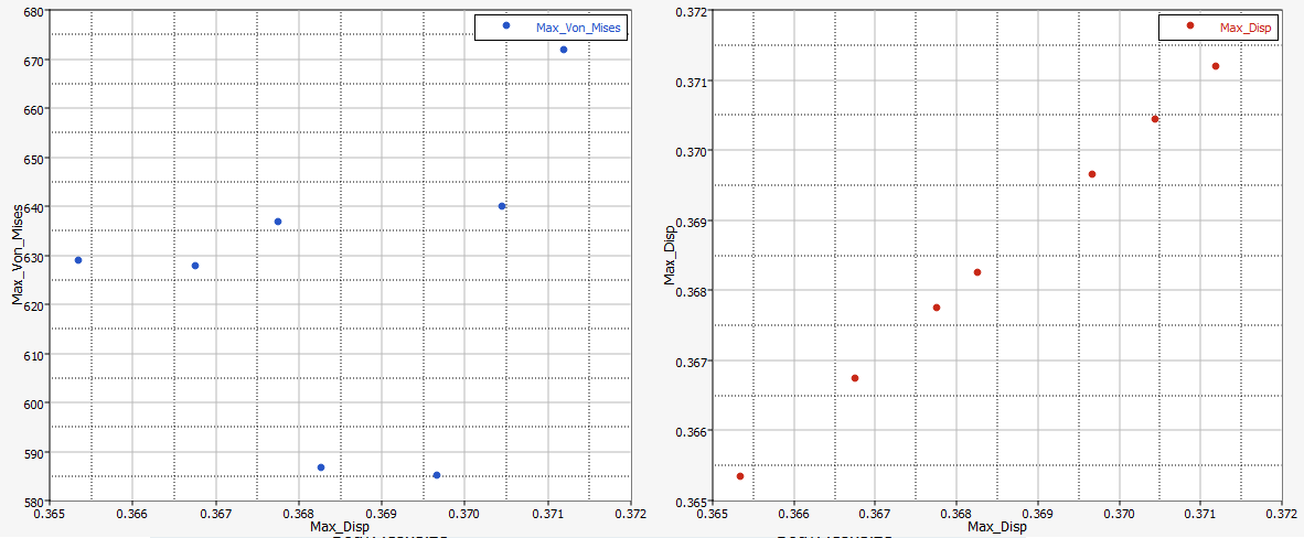
Click the Scatter tab.
From the Channel selector, set the X Axis to
BodyMeshSize and the Y Axis to
Max_Von_Mises and
Max_Disp.
The results of the scatter plot indicate that as the size of the mesh
gets smaller (moving along the x-axis to the left), displacement
starts to converge. However, stress does not converge. This behavior
is typical in finite element models when displacement converges
before derived quantities such as stress. In this tutorial, the
Max_Von_Mises output response may not converge at all due to the
location of the maximum stress in the model (adjacent to the load
application area), which can be seen by opening the resulting file
in HyperView.Figure 4.


 .
.
 .
.