Since version 2026, Flux 3D and Flux PEEC are no longer available.
Please use SimLab to create a new 3D project or to import an existing Flux 3D project.
Please use SimLab to create a new PEEC project (not possible to import an existing Flux PEEC project).
/!\ Documentation updates are in progress – some mentions of 3D may still appear.
Panel 1 : Static identification
Overview of the Static identification panel
MILS's first panel is depicted in Figure 1. It provides the user with nine actions or steps to complete a static LS identification, as indicated by labels 1.1 to 1.9 in that figure. The mandatory steps are labeled in blue, while the optional actions are displayed in yellow.

Mandatory steps in static identification
A static identification consists of a five-step procedure in MILS. The mandatory steps are described below:
- Step 1.1: Click on button Load measurements, which is labeled as
1.1 in Figure 1. MILS
will ask for measurement files. The user must here provide a set of measurement
files representing a certain number of static hysteresis loops of the steel
sheet. Each file in the selected set should correspond to a hysteresis loop
reaching a different magnetic flux density (until saturation).Note: The static hysteresis loop measurement files are text files that follow a specific format. A detailed description of MILS's input formats is available here.Note: If the files are loaded correctly, MILS will display the measurements provided by the user in the Curves preview window, as shown in Figure 2.
Figure 2. Hysteretic loop measurements displayed at the Curve preview window of the Static Identification panel in MILS. 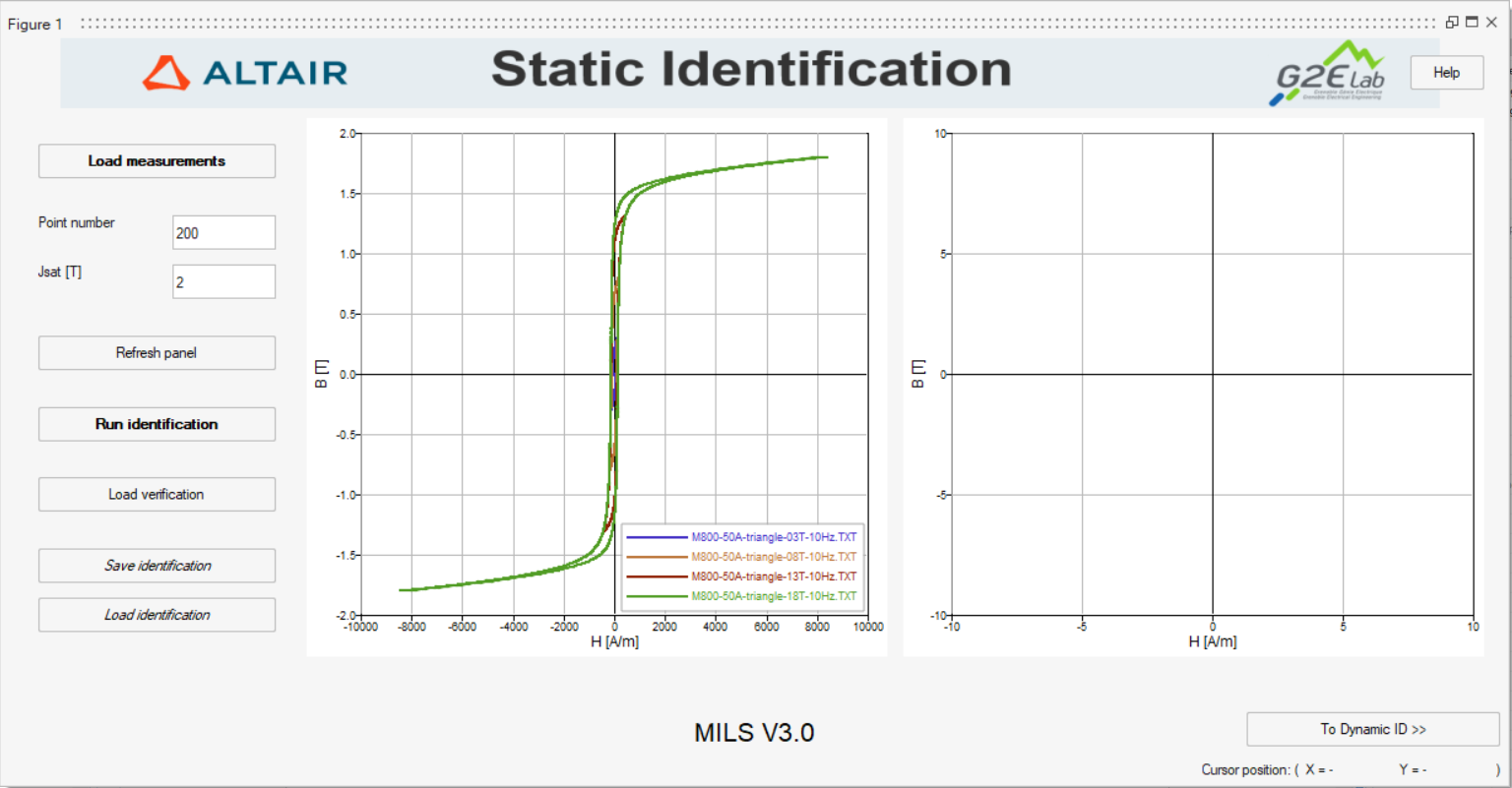
- Step 1.2: Provide an integer number in the field labeled as 1.2 in Figure 1. This number
represents the number of sampling points used to reconstruct a hysteresis
loop while evaluating the static component of the LS model. Note: The recommended values for this parameter are integers in the range between 100 and 500. While increasing this parameter improves accuracy, it also leads to longer processing times (not only during the identification but also during the actual evaluation of iron losses in Flux with the resulting LS model). The suggested default value (200) represents a good compromise between accuracy and speed.
- Step 1.3: Provide an initial estimation for the value of
Jsat, the saturated magnetic polarization of the steel
sheet in the field labeled as 1.3 in Figure 1. Note: The Jsat parameter is measured in teslas and may be obtained from an anhysteretic magnetization curve of a steel sheet as shown in Figure 3. Remark that MILS re-evaluates Jsat during the static identification, representing a corrected value that fits the measurement set.
Figure 3. Obtaining the saturated magnetic polarization of a steel sheet from the asymptotical behavior of its anhysteretic magnetization curve. 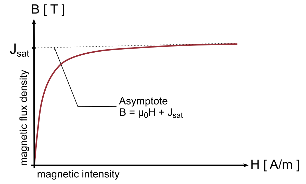
- Step 1.4: Launch the static identification by clicking on the Run
identification button, which is labeled as 1.4 in Figure 1.Note: The computation time required to complete the static identification is a function of the number of files loaded in step 1.1. Long identification times may be observed in the case of a large set of input files. A pop-up window appears at the end of the computation to announce the end of the static identification procedure, as shown in Figure 4.
Figure 4. The pop-up message announcing the end of a successful static identification. 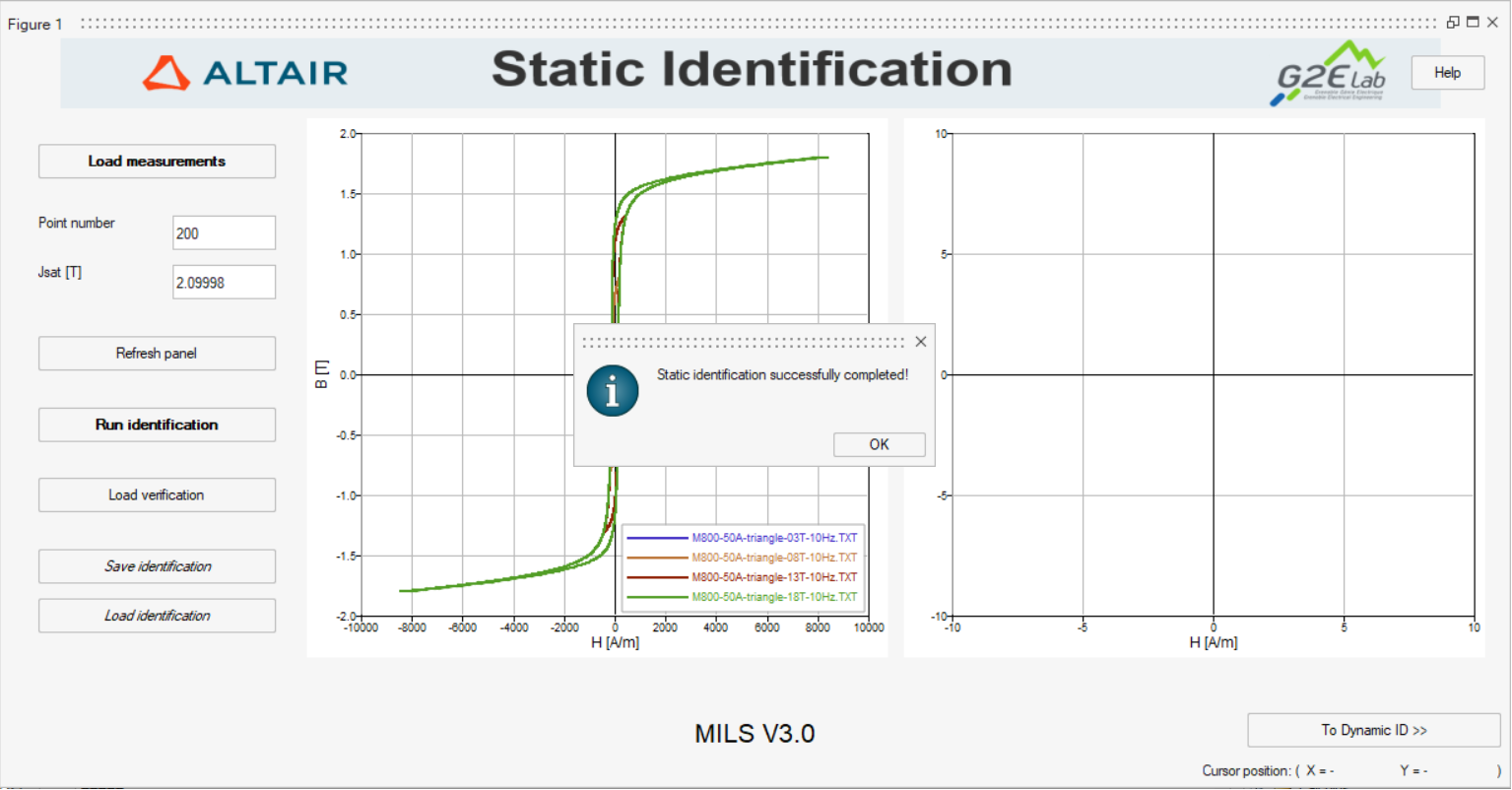
- Step 1.5: Once the static identification completes, click on button To Dynamic ID (labeled as 1.5 in Figure 1) to continue to the Dynamic Identification panel of MILS and proceed with the LS model identification.
Optional actions in static identification
- Refresh Panel: Clicking on button Refresh Panel (labeled as 1.6 in Figure 1) refreshes the Curve preview and Verification windows. Use this action to reset zoom settings and to change the colors of the displayed data sets in those windows.
- Verification: After completion of the mandatory steps 1.1 to 1.4, an
optional verification of the static part of the LS model may be performed. This
verification consists of reconstructing one or more hysteresis loops (given as
an additional set of measurements) using the identified static LS model and by
comparing their associated magnetic losses. To do so, click on button Load
verification (labeled as 1.7 in Figure 1). This action
will open a dialog box asking for an additional set of measurement files. Note: In this verification step, the user may choose between loading the same measurement set used in step 1.1 or a different one. In any case, MILS uses the identified static model to reconstruct a hysteresis loop for each file, by admitting a B(t) input issued from the loaded file.Note: MILS plots the reconstructed hysteresis loops yielded by the static LS identification in red in the Verification window of the static identification panel. The measurements loaded for verification are also plotted for comparison.Note: MILS estimates the error in the evaluation of the static component of the iron losses by comparing areas of the hysteresis loops. The percent error between the identified model and a measurement file is displayed in the legend of the Verification window, as shown in Figure 5.
Figure 5. Verification of a static identification computation in MILS. 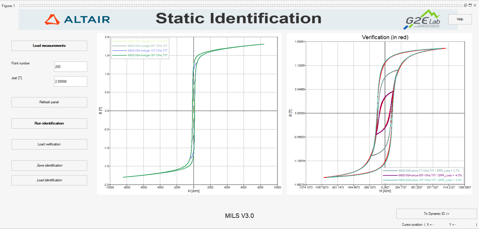
- Save or Load Identification: After completing steps 1.1 to 1.4, the user may save the static identification results for a later user by clicking on button Save Identification, marked as 1.8 in Figure 1. The saved results are stored in a MAT file (i.e., in Compose's workspace format). Conversely, a MAT file containing static identification results may be loaded by clicking on button Load Identification (labeled as 1.9 in Figure 1).
Further reading
LS model identification with MILS
How to use MILS to generate an LS model
Panel 2: Dynamic Identification
Panel 4: Model generation for Flux
MILS's input and output files formats
Bibliographical references on the LS model
Isotropic soft magnetic material: iron sheets described by LS model