Iron losses: à posteriori LS model

Loss surface model

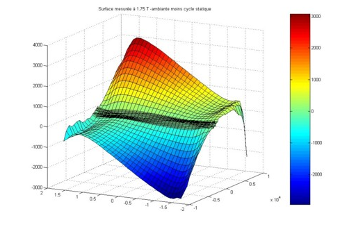
The Loss Surface (LS) model in Flux allows the evaluation of iron losses in magnetic cores composed by stacks of electrical steel sheets, i.e., described by Laminated magnetic non conducting regions. This model is based on the experimental observation that the losses in an electrical steel sample may be expressed as a function of two variables: the maximum value of the magnetic flux density (which is supposed to vary periodically in time) and the time derivative of the magnetic flux density. This function may be regarded as a surface in the 3D space, the Loss Surface of the material.

Consequently, for a given electrical steel grade, this function may be mapped experimentally through a convenient set of magnetic measurements that sweeps the 2D domain of this function. To achieve this, several combinations of magnetic flux density peak values and time-derivative values are needed and a dedicated magnetic measurement bench is required. The Epstein-type bench must be able to drive the magnetic flux density in time to obtain triangular waveforms (i.e., with a constant time derivative), with different peak values and at various frequencies.

An example of characteristic surface H(B,dB/dt) obtained from measurements is shown in the figure below:

Once this Loss Surface is completely mapped, it becomes possible to use it to create an empirical model of hysteresis for the electrical steel sheet: which Flux relies on to reconstruct in post-processing operations, in each point of the material, the B(H) loop an example of which is represented in the figure below: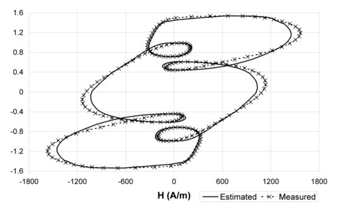

This model accounting for both static and dynamic hysteresis phenomena, allows then evaluating from B and H fields (homogenized through the stacking factor ${\lambda }_F$ ) the iron losses à posteriori in a Flux project in a fashion much similar to that given by the modified Bertotti model.

The advantage of the Loss Surface approach is that the model may be identified for a specific batch of electrical steel sheets used by a manufacturer, leading to very accurate results (under the condition that the measurements and the identification of the model have been done correctly). Users interested by this approach (i.e., who want to perform their own magnetic measurements to identify their own Loss surface models for their sheets) must also use the Loss Surface model identification tool provided in Flux, which is known as MILS. Further information is provided in the following user guide page: LS model identification with MILS.

On the other hand, users who cannot or who do not want to make their own magnetic measurements to identify the LS model representing their sheets may rely on the pre-identified models available out-of-the box in Flux for several electric steel grades. The list of available grades is given at this page.

Usage of LS model in Flux

An LS model in Flux can only be applied to Laminated magnetic non conducting regions and is only available in Transient Magnetic applications (2D, 3D and Skew).