Evaluating iron losses à priori in magnetic cores

Introduction

This page deals with the computation of iron losses in magnetic cores whose material is defined in a Flux project by one of the Preisach models:

Isotropic hysteretic, Preisach model described by 4 parameters of a typical cycle and
Isotropic hysteretic, Preisach model identified by N triplets

or by the Jiles-Atherton one:

Isotropic hysteretic, Jiles-Atherton model

The materials having these types of B(H) property take into account ferromagnetic hysteresis phenomena during the resolution of the project and so, they allow a direct or a priori evaluation of hysteresis and iron losses in the ferromagnetic materials.

The following subjects are covered in the next sections:

Static and dynamic hysteresis
Evaluating hysteresis and iron losses in Flux with a hysteretic material
Application example
Bibliographical references

Static and dynamic hysteresis

During their operations, several parts of electromechanical devices are subjected to time-varying magnetic fields, which generate - in the volumes made of ferromagnetic materials exhibiting a hysteretic behavior - the so-called hysteresis losses: in fact, during the demagnetization processes the material does not give fully back the energy stored during magnetization phases, but it dissipates part of this energy in the form of heat.

Moreover, the magnetic field variations induce - in the conducting volumes - eddy currents (also called Foucault currents) which result in losses via the Joule effect. These two contributions create what is usually referred to as iron losses which are identified by the following general expression:

$dP = H . \frac{\partial B}{\partial t} + ρ J^{2}$ (1)

where:

dP: the iron loss density (W/m³) ;
H: the magnetic intensity (A/m) ;
B: the magnetic flux density (T) ;
ρ: the electrical resistivity of the material (Ω.m) ;
J: the induced current density (A/m²).

In (1), the two aforementioned contributions can be clearly distinguished. In case of slowly varying fields, the Joule losses term $ρ J^{2}$ is small because the induced currents are negligible and the losses are almost purely hysteretical in nature. On the other hand, when the time rate of change of the fields increases (i.e. the frequency increases), both the hysteresis losses and the Joule losses tend to increase.

To represent graphically this behaviour, another expression - similar to (1) - for the iron loss density dP can be derived by using measurable macroscopic quantities (further details in the bibliographical references at the end of this page):

$dP = Hs . \frac{\partial Ba}{\partial t}$ (2)

where:

dP is the iron loss density in the region (W/m³) ;
Hs is the surface magnetic intensity on the region (A/m) and
Ba is the average magnetic flux density in the cross section of the region (T).

The unique term on the right hand side of this equation (2) accounts for both hysteresis and eddy current losses, because Hs and Ba are functions of the overall distribution of the fields in the region (including the contribution arising from eddy currents at higher frequencies) and so the term $Hs . \frac{\partial Ba}{\partial t}$ accounts for the full iron losses and not only for the hysteresis losses.

It follows from the above that the area enclosed by the hysteresis loop of Ba(Hs) (see figure below) represents the total energy dissipated in a cycle (i.e. the sum of both hysteresis and Joule effect contributions):

at low frequencies, the hysteresis cycle is narrow due to negligible induced currents and Joule losses: these circumstances are usually referred to as static hysteresis;
at higher frequencies, the hysteresis cycle Ba(Hs) widens due to the development of induced currents leading to Joule losses: these situations are identified as dynamic hysteresis.

Figure 1. Static hysteresis cycle (at 10 Hz, in red) and dynamic hysteresis cycle (at 1000 Hz, in blue) in a magnetic region subjected to eddy currents.

Evaluating hysteresis and iron losses in Flux with a hysteretic material

In a Flux project containing a Transient Magnetic application, the user may choose between two approaches to evaluate iron losses during the resolution:

Represent static hysteresis only: a material containing a hysteretic B(H) property based on the Preisach or the Jiles-Atherton models must be defined and assigned to a magnetic non-conducting region. This approach is well-adapted for low frequency problems.
Include dynamic hysteresis, i.e. evaluate increased iron losses due to eddy currents: the material containing a Preisach or Jiles-Atherton B(H) property must also have a J(E) property and be assigned to a solid conductor region instead of a magnetic non-conducting region.

In the first case (i.e., static hysteresis: material with B(H) property and magnetic non-conducting region), Flux provides the user with the quantity dPowMagV:

which is available in the formula editor under the button dPowerMag / dV to be used for graphical displaying of the magnetic power density (i.e. the hysteresis loss density) in post-processing (e.g. isovalues);
and which can be integrated over the region volumes by means of a Sensor to get the whole dissipated power associated to the static hysteresis (i.e., the hysteresis losses):

To this aim the user must:

create a Sensor through the menu Parameter/Quantity or Computation depending if the project is not solved yet or already solved, respectively;
choose Predefined as type of sensor;
and Magnetic power as quantity to compute;
select the magnetic non-conducting regions with a hysteretic B(H) property;
evaluate the sensor.

In the second case (i.e. dynamic hysteresis: material with both B(H) and J(E) properties and solid conductor region), Flux provides the user with the quantity dPowV:

which is available in the formula editor under the button dPower / dV to be used for graphical displaying of the total power density (i.e. the iron loss density) in post-processing (e.g. isovalues);
and which can be integrated over the region volumes by means of a Sensor to get the whole dissipated power associated to the dynamic hysteresis (i.e., the iron losses):

To this aim the user must:

create a Sensor through the menu Parameter/Quantity or Computation depending if the project is not solved yet or already solved, respectively;
choose Integral as type of sensor;
select the solid conductor regions containing the hysteretic B(H) property and a conductivity model J(E);
in the field Spatial formula, select the quantity dPower / dV in the formula editor;
evaluate the sensor.

The table below summarizes the two modeling approaches described in this section.

Table 1. Summary of the calculation of hysteresis and iron losses for a hysteretic model.
Material	Active property	Region	Computation method	Evaluated quantity
Hysteretic Isotropic Material characterized by a Preisach-type model or Isotropic soft magnetic material: hysteresis Jiles-Atherton model	B(H)	Magnetic non-conducting	Predefined sensor (type magnetic power) on a region (quantity dPowMagV)	Hysteresis losses
	B(H) and J(E)	Solid Conductor	Sensor evaluating the integral of the quantity dPowV on a region	Iron losses

Application example

Let's consider once again the TEAM 32 problem presented in this page and let's use it to compare the evaluation of iron losses with the two previously discussed approaches, namely:

the static hysteresis approach: based on a material containing a Preisach B(H) property assigned to a magnetic non-conducting region;
the dynamic hysteresis approach: based upon a material containing both a Preisach B(H) property and a isotropic linear J(E) property assigned to a solid conductor region.

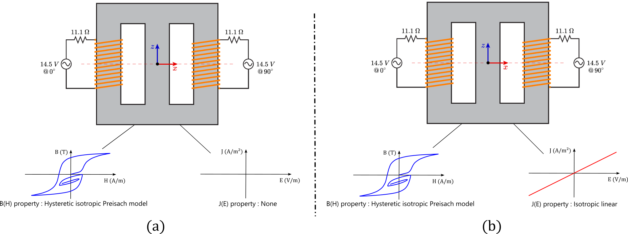
The application of these two approaches to the TEAM 32 problem is summarized in the figure below:

Figure 2. 2D representation of TEAM 32 problem with (a) the approach with a non-conducting magnetic region and a hysteretic B(H) property and (b) the approach with a solid conductor region, a hysteretic B(H) property, and an isotropic linear J(E) property.

The two voltage sources that feed the circuit impose a sinusoidal voltage with an amplitude of 14.5 V and a phase shift of 90° between these them. Several computations were performed, with the frequency of the voltage sources going from 1 to 100 Hz and with both approaches. The goal is to compare the hysteresis losses with the total iron losses for each frequency.

After resolution, a comparison between the two previous approaches may be performed by comparing the total iron losses with the hysteresis losses, as shown in the figure below:

Figure 3. The total power dissipated in the magnetic core as a function of the supply frequency. The orange line corresponds to the approach based on a non-conducting magnetic region and a material with hysteretic B(H) property. The blue line on the other hand corresponds to the approach using a solid conductor region and a material with hysteretic B(H) and linear isotropic J(E) properties.

The eddy current distribution may be visualized through an arrow plot of the current density J in the magnetic core, as shown in the figure below.

Figure 4. Distribution of induced currents evolving in the volume of the magnetic core evaluated with the approach based on a solid conductor region, a hysteretic B(H) property and an isotropic linear J(E) property.

Bibliographical references

H. Pfützner and G. Shilyashki, "Theoretical Basis for Physically Correct Measurement and Interpretation of Magnetic Energy Losses," in IEEE Transactions on Magnetics, vol. 54, no. 4, pp. 1-7, April 2018, Art no. 6300207, doi: 10.1109/TMAG.2017.2782218.
M. Tousignant. Modélisation de l’hystérésis et des courants de Foucault dans les circuits magnétiques par la méthode des éléments finis. Energie électrique. Université Grenoble Alpes; Polytechnique Montréal (Québec, Canada), 2019. (in French). ⟨NNT : 2019GREAT065⟩. ⟨tel-02905410⟩