Iron losses: à posteriori Bertotti model

The modified Bertotti model

The Bertotti model implemented in Flux is a modified version of the well-known standard Bertotti model for iron losses. These models belong to the larger family of Steinmetz-like methods that establish empirical relationships between the specific losses (in W/kg) in an electrical steel sheet and the frequency of the magnetic flux density in the material.

Since hysteresis phenomena, which are the cause of iron losses, require a time-domain representation, the standard Bertotti model is reformulated in Flux to apply it to non-sinusoidal waveforms, to provide the users with more degrees of freedom, to account for possible non-zero continuous components of B and to unify the equations and the parameters to use for both transient and frequency domains. Due to these specificities, the implementation of the Bertotti model in Flux is said to be 'modified': in other words, it has been tailored or optimized to work robustly in the context of Finite Element computations.

Accordingly with the modified Bertotti model, the iron loss density (directly related to the specific losses by the mass density) in a stack of electrical steel sheets may be decomposed in a sum of three terms: namely hysteresis, classical (also called eddy current) and excess losses terms. In each point of the material described by a laminated magnetic non conducting region, in the frequency domain the following equation holds:

where

represents the mean iron loss density, in W/m³;
$λ_{F}$ is the stacking factor of the lamination;
$k_{1}$ is the hysteresis losses coefficient;
$α_{1}$ is the hysteresis losses exponent;
$k_{2}$ is the classical losses coefficient;
$α_{2}$ is the classical losses exponent;
$k_{3}$ is the excess losses coefficient;
$α_{3}$ is the excess losses exponent;
$f_{}$ is the frequency of the magnetic flux density, which is supposed to vary periodically in time;
$B_{max}$ (in teslas) is the maximum magnitude that the homogenized magnetic flux density can reach in the considered point of the laminated region over a period ${T=1/f}_{}$ ; this value is automatically computed by Flux through the magnetic flux density and the stacking factor $λ_{F}$ .

Similarly, in the time domain the following equation holds:

where

represents the instantaneous iron loss density, in W/m³;
T is the period of the magnetic flux density;
and are the maximum excursions from their continuous component, of the longitudinal and the transversal projections of the homogenized magnetic flux density over the period T, respectively; in each point of the laminated region, the longitudinal direction is defined as the direction of B at the time step where the magnetic flux density reaches its maximum value during the considered period, while the transversal direction is orthogonal to the longitudinal one, as shown in the image below;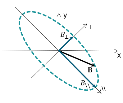
is the magnitude of the time derivative of the homogenized magnetic flux density, which has been beforehand decomposed into its longitudinal and transversal projections defined here above;
the coefficients $k_{i}$ and the exponents $α_{i}$ are the same as in the frequency-domain equation above.

In both above equations, the first term referred to as hysteresis and characterized by the parameters $k_{1}$ and $α_{1}$ , represents the static hysteresis phenomena and enables to evaluate the so-called hysteresis loss density (see this page for more information). The second and third terms referred to as classical (or eddy current) and excess, respectively, account also for the dynamic hysteresis phenomena, so that the whole modified Bertotti equation enables to evaluate the full iron loss density.

The coefficients $k_{i}$ and the exponents $α_{1}$ above are specific to a given electrical steel grade or sheet type. They are typically determined by a curve-fitting procedure on magnetic measurement values provided by manufacturers in data sheets (i.e., a table of specific losses measured as a function of the magnetic flux density $B_{max}$ at several frequencies). To help users for determining the Bertotti model parameters, Flux provides a Material Identification tool, based on Compose language.

Based on the iron loss density in all points and the Finite Element shape functions, Flux efficiently integrates this quantity in the volume of the laminated magnetic non conducting regions to compute the à posteriori iron losses.

Usage of modified Bertotti model in Flux

Since the modified Bertotti model is only used during post-processing operations, it is a complementary definition to be added to the B(H) characteristic of the soft material of the region. The Bertotti parameters can be filled:

either in the Material dialog box, in the dedicated Iron losses tab, where the user has to check the Model for iron losses computation box and then define the values for the Coefficients and for the Exponents in the corresponding sub-tabs;
or during post-processing phases through the dialog box provided for the iron losses computation on regions or the multiparametric one.

In Flux, the modified Bertotti model is available in 2D, Skew and 3D modules for all Magnetic applications, i.e., Transient, Steady State AC and Static (in Advanced Mode only for the latter) and can only be applied to Laminated magnetic non conducting regions.