Since version 2026, Flux 3D and Flux PEEC are no longer available.
Please use SimLab to create a new 3D project or to import an existing Flux 3D project.
Please use SimLab to create a new PEEC project (not possible to import an existing Flux PEEC project).
/!\ Documentation updates are in progress – some mentions of 3D may still appear.
The temperature coefficient
Introduction
- their counterpart models non-dependent on the temperature
- plus a coeff(T) temperature coefficient, built on the basis of two exponential functions (detailed description in the following paragraphs)
Mathematical model
- the first, with a negative decay rate, is used when coeff(T) ranges from 1 to 0.1, which means up to a temperature T* equal to TC - 0.10536 C, where C is the inverse of the exponential decay constant of the material
- the second, with a positive decay rate, is used in the neighborhood of the Curie point, when coeff(T) ranges from 0.1 to 0, which means beyond the temperature T*
From a mathematical point of view, the model for the coeff(T) function can be written as follows:

where the temperature T, the Curie temperature TC, as well as C (the inverse of the exponential decay constant of the material) are expressed in degrees Celsius °C. The coefficients
 and
and 
are determined so that the two exponentials can connect at the point where coeff(T*) = 0.1
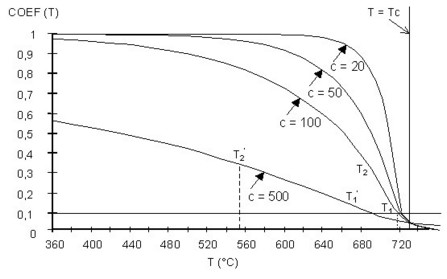
Being the exponential decay constant of the second function ten times greater than its counterpart of the first exponential, at the temperature T* both exponential functions take the same value, thus ensuring the continuity of the global coeff(T) model, as illustrated in the figure below.

Model parameters
- the material Curie temperature TC, which can be found in manufacturer's data-sheets
- and C, which is the inverse of the exponential decay constant of the material and can be considered a sort of temperature constant to describe how fast the material loses its magnetic properties when the temperature increases.
The figure below plots the coeff(T) function for TC = 727 °C and several values for the parameter C to illustrate its impact on the temperature-dependent material properties. The lower the value of C, the more the material retains its magnetic properties at temperatures close to the Curie point.