Steps for iron losses computation on regions

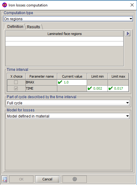
In the Computation type drop-down menu, choose option On regions.

Select the desired laminated regions for iron losses computation by filling the list.

Proceed by choosing or fixing:

The values of geometric and I/O parameters to consider for the iron losses computation.
In the case of Transient Magnetic applications, the time interval over which the iron losses have to be evaluated from the computed magnetic flux density B(t) values over the same period. Flux interprets B(t) over this time interval accordingly with the option selected in the Part of cycle described by the time interval drop-down menu.

Attention: In order to obtain physically meaningful results, the user must choose the correct time interval that accords with the Part of cycle described by the time interval option discussed below. For instance, with the option Full cycle the user must select a time interval corresponding to one and only one electrical period of the device; similarly, with the option Half cycle he must select a time interval corresponding to a half electrical period.

The option Part of cycle described by the time interval, whose available interpretations are described in the table below:

Option	Description
No cycle	To compute iron losses, Flux uses the magnetic flux density B(t) obtained during the provided time interval with no assumption regarding the periodicity of the waveforms. Consequently, Flux does not display any warning or error message in case of a non-periodic B(t) waveform.
Full cycle	Flux interprets the provided time interval as a full electrical period. More specifically, Flux checks the periodicity of the magnetic flux density B(t) by comparing its values at the first and last time steps of the selected interval. Then, if the periodicity tests fail, Flux displays a warning message, but the computation is nevertheless carried out.
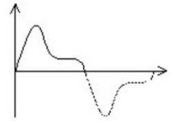
Half cycle (available only in advanced mode)	Flux interprets the provided time interval as a semi-period and reconstructs the B(t) signal along the second missing semi-period by considering its waveform as antiperiodic, as shown in the picture below. Then, Flux uses the complete reconstructed B(t) waveform to compute the iron losses. Note: This Half cycle option is well-adapted for cases in which the B(t) waveform has a non-zero mean value (off-set).

Note: The first two time steps of a scenario can not be selected for the definition of the time interval and are hidden from the list.

Note: With the Full cycle and Half cycle options, Flux will also evaluate a parameter indicating if the selected time interval corresponds to a periodical magnetic flux density. This parameter is called Error on periodicity (in %) and is available together with the iron losses result, in the computation result dialog box (for further information, see Results of iron losses computation on regions).

Note: In case of periodic waveforms and while using the Modified Bertotti model (see step 4 below: Model for losses), both options No cycle and Full cycle provide quasi identical results; minor differences may arise due to the numerical scheme. On the other hand, while using the Loss Surface (LS) model, and depending on the B(t) waveform on the selected time interval, the No cycle option may not always use a full, closed hysteresis cycle to perform the computation, thus leading to potentially non-negligible differences when compared to the Full cycle approach (which is consequently more accurate).

Finally, select the iron losses model in the Model for losses drop-down menu. The following options are provided:

Model defined in material: the iron loss model defined in the material assigned to the region is employed for the computation.
Modified Bertotti: with this option, the user must provide the coefficients and exponents required to fully describe the Modified Bertotti model.
LS predefined sheets (in Transient Magnetic applications only): in this case, the user is asked to select from the drop-down menu an electrical steel sheet with a predefined Loss Surface (LS) provided with Flux.
LS defined by importing of a MILS file (in Transient Magnetic applications only): in this case, the user needs to provide his own Loss Surface model of an electric steel sheet as a .MILS file. For further information on how to create such a file from magnetic measurements, see LS model identification with MILS).