Parabolic Equation (PE) Model

The parabolic equations model employs numerical evaluation of the parabolic equation (PE) to compute the field strength in a macro-cellular area based on terrain data.

The different propagation mechanisms (free space propagation, reflection and diffraction) are implicitly considered for the PE model resulting in an accurate model. Due to the sophisticated algorithm, the computation time is quite long in comparison to the empirical models.

Consideration of Propagation Phenomena

As the parabolic equations uses numerical algorithms to consider propagation phenomena like reflection and diffraction, it requires a long computation time, but it is an accurate model.

The PE model takes the following effects into consideration:

reflection
diffraction
forward-scattering

It accounts for the properties of the ground by the following parameters:

conductivity of the ground
dielectric permittivity of the ground

The standard parabolic equation (SPE) is a partial differential equation and is derived from the Maxwell equations, neglecting backward propagation and assuming a rotation symmetrical problem.

(1)

\frac{\partial Ψ}{\partial r} + \frac{j}{2 k_{0}} \cdot \frac{\partial^{2} Ψ}{\partial z^{2}} + j \cdot \frac{k^{2} - k_{0}^{2}}{2 \cdot k_{0}} \cdot Ψ = 0

$Ψ$ is the field strength related to field of a linear source. In the far field the vertical component of the electrical field can be assumed as

(2)

E_{z} = Z_{F_{0}} \cdot H_{Φ} \frac{ψ}{\sqrt{r}} \cdot e^{- j k_{0} r}

where Z_F0 is the wave impedance and k₀ denotes the wave number in free space while k is the complex wave number in an inhomogeneous lossy atmosphere.

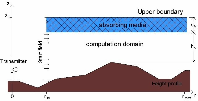
The results of the PE are only valid, if the propagation angle in respect to the horizon lies within -15° up to +15°. This is reason why the computation starts at the distance rini.

Some of the upper layers of the atmosphere have the effect like a reflector. As the reflected waves increase the computation time, an absorbing medium below these layers is assumed. The height of the absorbing medium is about dA = 150 wavelengths.

PE has three possibilities to consider the conductivity and the dielectric permittivity of the ground soil;

discrete terrain approximation
continuous terrain approximation
terrain profile approximation with coordinate transformation

With an extension of the SPE, the disadvantage of the rather small propagation angle can be avoided. The so-called wide angle parabolic equation (WAPE) model leads to valid results for propagation angles between -40° up to +40°. As this extension is not noticeable in the computation time, the WAPE should be preferred.

Settings

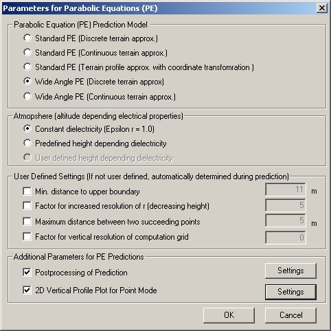
ProMan offers five variations of the parabolic equation model. They differ in the underlying parabolic equation type and the implementation of the impedance boundary at the ground. The standard choice is the wide angle PE (discrete terrain approximation) which leads to good results for all types of terrain.

Standard PE (Discrete terrain approx.)

This variation applies the standard PE and does a discrete approximation of the height profile. For decreasing heights the iteration step size is reduced in an adaptive way to avoid prediction errors caused by the imperfect boundary condition for down-sloping grounds.

Standard PE (Continuous terrain approx.)

This variation is based on variation 1. However, the impedance boundary is replaced by a continuous modeling of the height profile, which does not improve the prediction quality but the stability of the iteration algorithm.

Standard PE (Terrain profile approx. with coordinate transformation)

A transformation of the vertical coordinate is used to get a rectangular computational domain for the PE discretization grid. No additional efforts had to be taken to handle the trouble at down-sloping ground. Thus, the iteration step size is constant. This model should only be used for slight hilly terrains. The transformation results in a computation time that is about 50% higher than that of all other variations.

Wide Angle PE (Discrete terrain approx.)

The standard PE is extended to a wide-angle form, allowing larger propagation angles with respect to the horizon. Having nearly the same computation time as variation 1, this option should be preferred.

Wide Angle PE (Continuous terrain approx.)

This variation is the wide-angle extension of 2.

Atmosphere

The option Constant dielectricity performs a free-space simulation while the option Predefined height depending dielectricity assumes a standard atmosphere based on the following formula:

(3)

n = 1 + 0.000315 * e^{(- 0.000136 * z)}

with z in m.

User Defined Settings

If the following options are left cleared, ProMan sets the appropriate values at run-time (recommended).

Min. distance to upper boundary: Defines the distance between the highest terrain point (includes the transmitting antenna) and the upper boundary of the regular computation domain in the vertical terrain section.
Factor for increased resolution of r (decreasing height): This factor influences the radial iteration step size at down-sloping ground. Greater values lead to smaller iteration steps. Recommended values are 3 for hilly and 1 - 2 for mostly flat terrain
Maximum distance between two subsequent point: Sets the radial iteration step size for flat and rising ground. The PE variation 3 uses this step size for all slopes.
Factor for vertical resolution of computation grid: Sets the vertical grid size of the computation grid in relation to the wavelength. Appropriate values are from 0.1 to 0.5.

Additional Parameters for PE Predictions

All PE models use a forward iteration algorithm. Therefore, backward orientated effects (such as reflections at the opposite hillside) are not considered. This leads to pessimistic predictions above down-sloping ground. To avoid unrealistic high path loss values, two post-processing modes has been integrated which can be configured by clicking Settings.

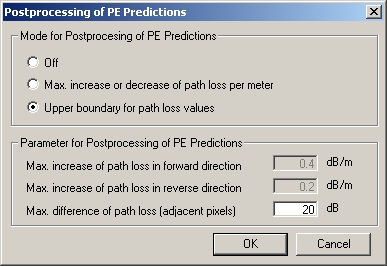
Mode for Post-processing of PE Predictions: The first option lets you turn the post-processing off. Activate the option Max. increase of path loss or decrease of path loss per meter, if you want to limit the path loss alterations by setting maximal values for the derivation path loss by range. Having selected the option Upper boundary for path loss values, extreme values of the path loss will be cut down on a value relative to that of the adjacent pixels.
Parameter for Post-Processing of PE Predictions: You can customize the PE post-processing parameters with the edit controls.

For test or illustration purposes it might be helpful to output the electromagnetic field above a vertical terrain section. This can be done by activating the 2D Vertical Profile for Point Mode of the PE check box. Furthermore, one single prediction point must be set, which defines the endpoint of the vertical section. ProMan then saves the field strength, power and pass loss (depending on your selection in the Output dialog) to a file denoted with the suffix “c-plot”.

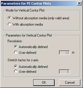
Mode for Vertical Contour Plot: The PE model appends an absorption medium at the top of the computation area to avoid reflections from the upper boundary. Here you can specify, if you want to output the contour plot with or without the absorption medium.
Parameters for Vertical Contour Plot: The pixel resolution and stretch factor of the contour plot can either be defined automatically or by the user. A stretch factor > 1 will show the vertical structure of the predicted field more clearly by scaling the z-axis. Using the automatically defined option, ProMan sets the values as shown in table:

Table 1. Vertical contour plot settings.
Range of the Vertical Plot r_max [m]			Resolution [m]	Stretch Factor For Z-Axis
Bigger or Equal		Smaller	Resolution [m]	Stretch Factor For Z-Axis
	r_max	350	1	1
350	r_max	750	1	5
750	r_max	1500	1	5
1500	r_max	3000	2	10
3000	r_max	7500	5	10
7500	r_max	15000	10	10
15000	r_max	30000	20	20
30000	r_max	75000	50	20
75000	r_max		100	20