Order Cut Analysis
![]()
Order Cut Analysis
The goal of the Ordercut Utility is to help user to understand the order content of the rotating machines signal and ways to identify the physical phenomenon that is causing the problem. And further help in isolating the problematic patterns to resolve NVH issues.
Order Cut Analysis tool uses to visualize order cut analysis date using waterfall plot, 2D graphs, 3D graphs and force vector animation.
Options
Result Type
The following options are available under Result Type.
Global result: Select this option for global results for which order analysis results are available.
Local result: Select a node/element: Select a node or element for local results of the response for which order analysis results are available.
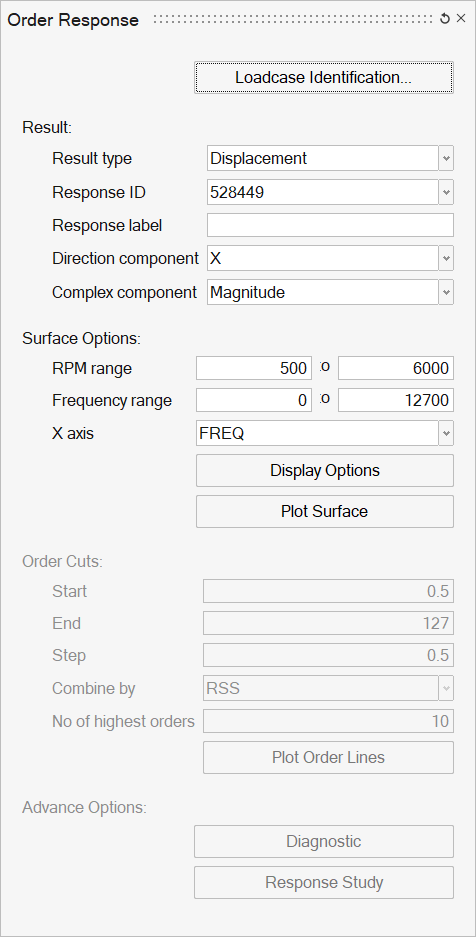
Result selectionThe following fields are available on the Order Response tab, under Result selection.
Result component: This field is populated based on global or local result types and selected entities from the file loaded. Select a result component for order analysis.
Response label (optional): Enter a label that describes the response, for example, "Left Engine Mount".
Direction component (optional): X, Y, Z, RX, RY, RZ, or XYZ Vector Sum.
Complex component: Magnitude or phase.
Range selection
Customize the RPM range and Frequency range fields as necessary.
Once your selections are complete, you can load the RPM-based response curves to generate a 3D surface plot.
Display Options: The Display Options dialog allows you to customize the surface plot, including scale, weighting, and the plot layout.
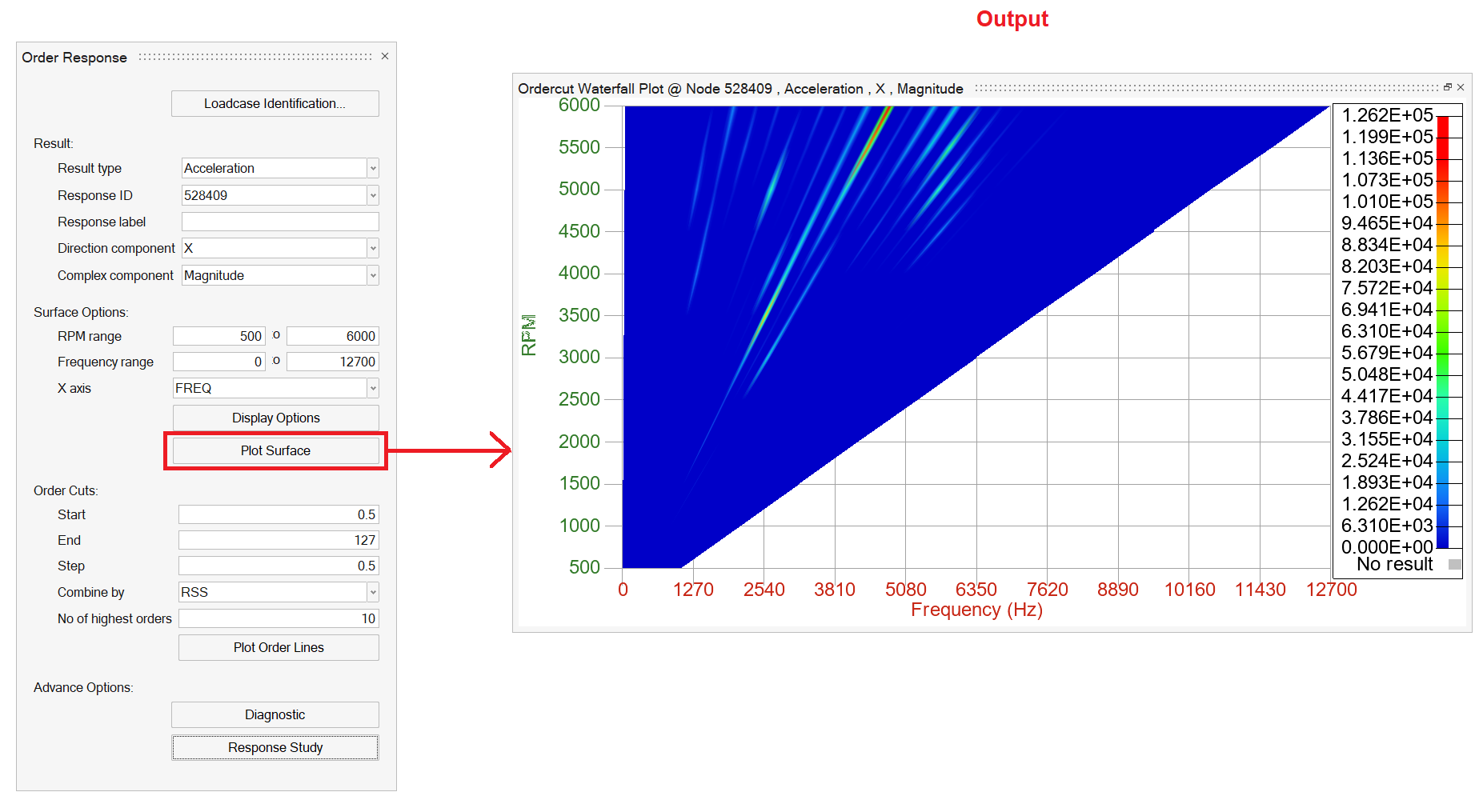
Plot Surface: Click to generate a 3D surface plot.
Order Cuts
After viewing the surface plot, use the Start, End, and Step fields to specify the orders you want to see by cutting the surface plot.
Combine Order By - Choose between RSS and Arithmetic Sum to determine how to combine the order curves to construct the overall response.
Display Options: The Display Options dialog allows you to customize the overall response plot, including scale, weighting, and the plot layout.
Load Response: Once your selections are complete, click Load Response to create the orders and order sum response overlay plot.
Select Subcase Group
The option to select radial, tangential, global, or moment group names which is available for all models.
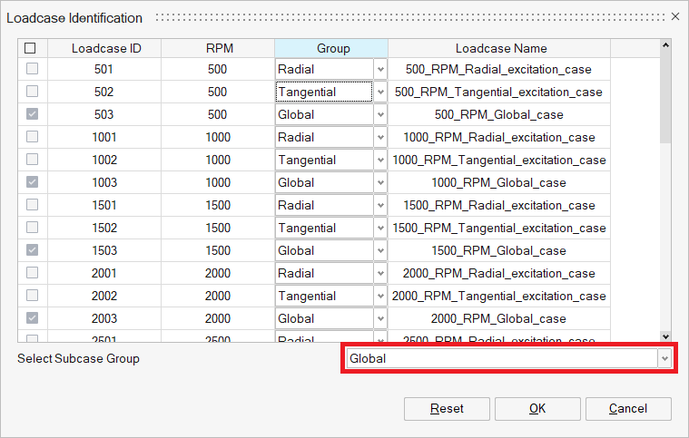
Reset: The LoadCase Identification Dialog can be reset to its original values using the Option.
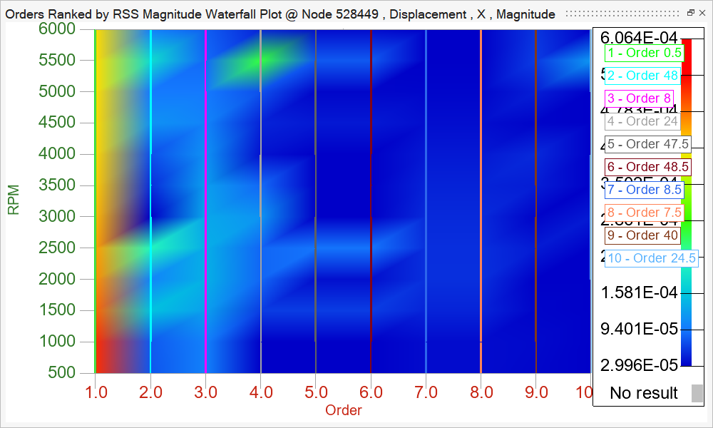
Plot Surface(Waterfall Diagram)
It gives user an overall or bird's-eye view of a particular response that can occur on an operating system. With frequency long x-axis & rotational speed along Y-axis and response amplitude along z-Axis.
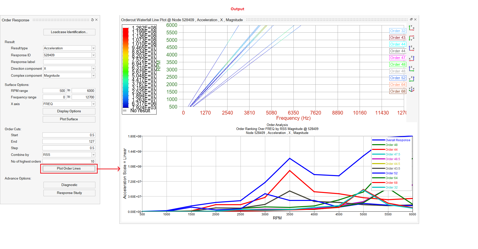
Plot Order Line
This uses to identify the Peak/Risk/Interest response.
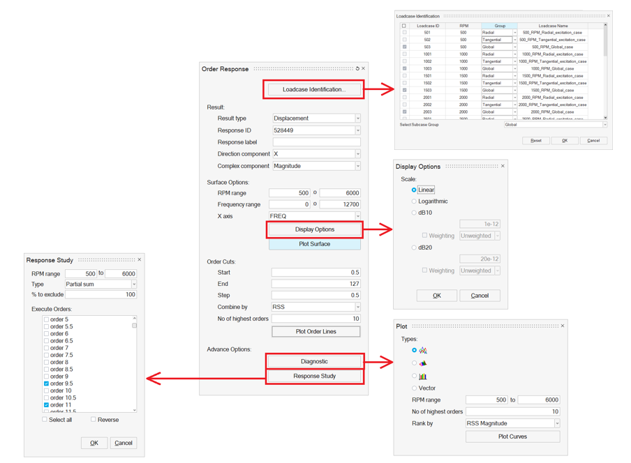
Diagnostic
Select a method to display and rank the orders.
- 2D
- 3D
- Bar
- Vector
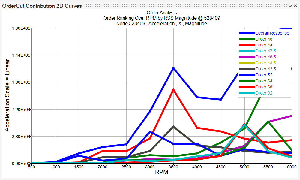
2D Plot
Shows peak points of response.
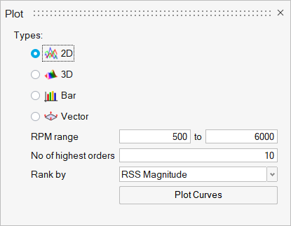
Display: Select the type of curve to display.
RPM range: Select the RPM range that the order curves should be plotted within.
No. of highest order: After defining the RPM range, organize the display by selecting the number of highest orders.
Rank by: Define the method that is used to rank orders with one of the following options:
-
Magnitude - Orders are ranked by the magnitude of the order. Available for Bar plot.
-
RSS Magnitude - Orders are ranked by the root sum of squares of the magnitude of the order at selected
frequencies. Available for 2D Line and 3D Surface plots.
Display Options:The Display Options dialog allows you to further customize the plot.
Display: Click <span class="ph uicontrol">Display</span> to create and display the plot.
Example
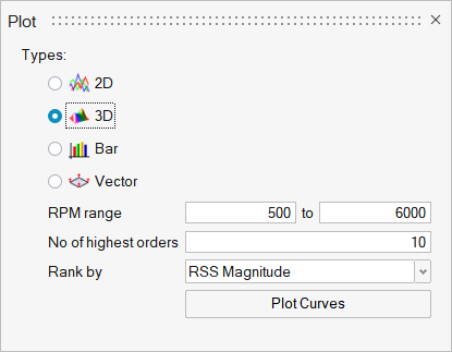
3D Plot
Creates a 3D Surface plot of the response within an RPM range.
RPM range indicates the available range, based on your results file.
Use the From and To fields to customize your own RPM range.
All other options are similar to those for the 2D Line plot.
Example
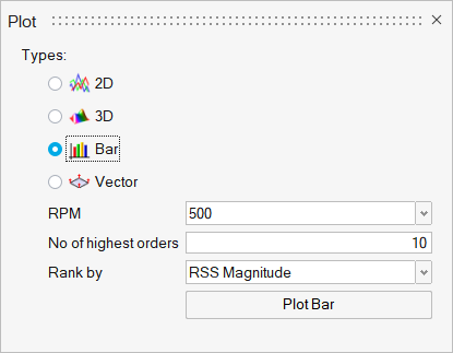
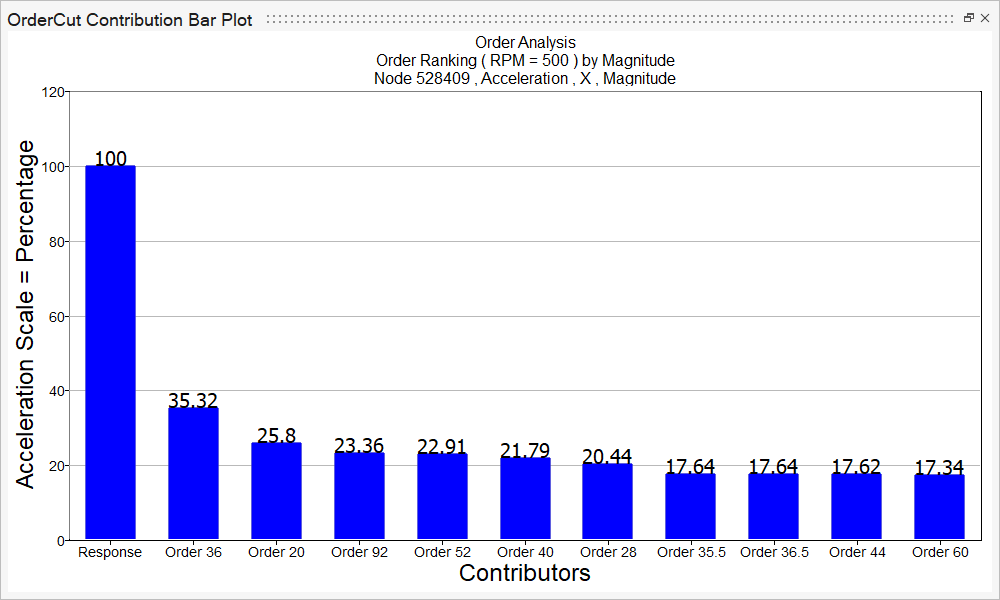
Bar
Creates a Bar plot of the response at a specific frequency or RPM.
Enter a specific RPM in the Specific RPM field, or use the slider bar to select an RPM value. When you use the slider bar to select an RPM, a red line is displayed on the response plot and is dragged simultaneously as you drag the slider bar.
All other options are similar to those for the 2D Line plot.
Example
Vector
Force vector animation.
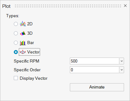
Specific RPM: Select the specific RPM for Vector animation.
Specific Order: After defining the RPM range, organize the display by selecting the specific orders.
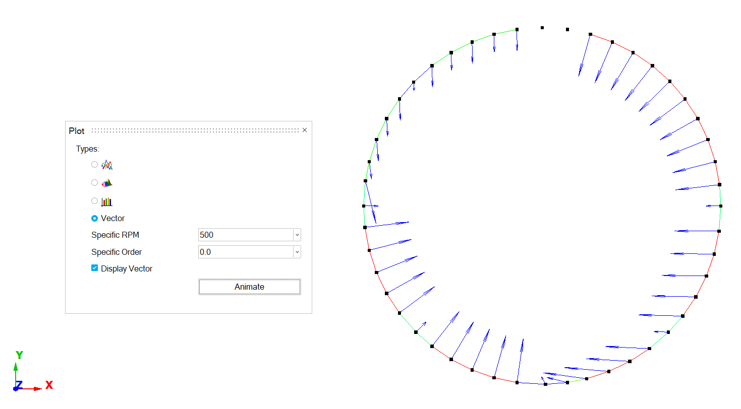
Display Vector: This option enables vector marker for animation.
Example
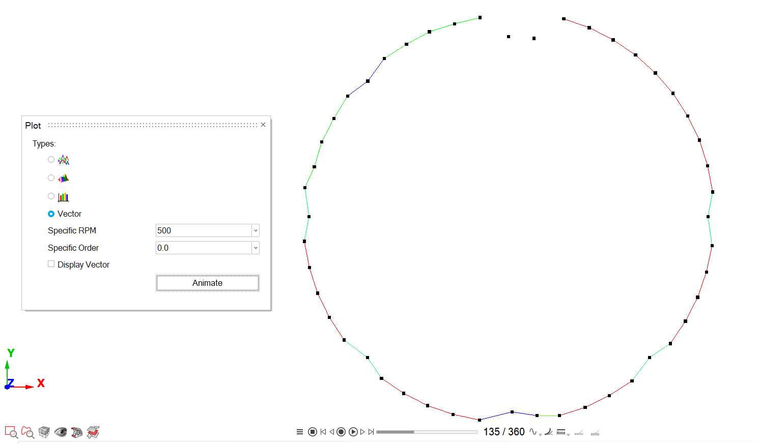
Example
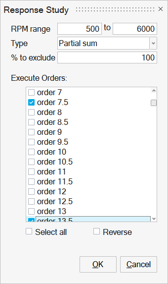
Response Study
Analysing the effect of Order on response.
After plotting the order analysis curves, perform a Partial sum or Order overlay response study.
Study/Curves over
Select the type of study to display. Choose between RPM or Frequency.
RPM RangeIndicates the available range, based on your results file.
Use the From and To fields to customize the RPM range.
Type
The type of response study.
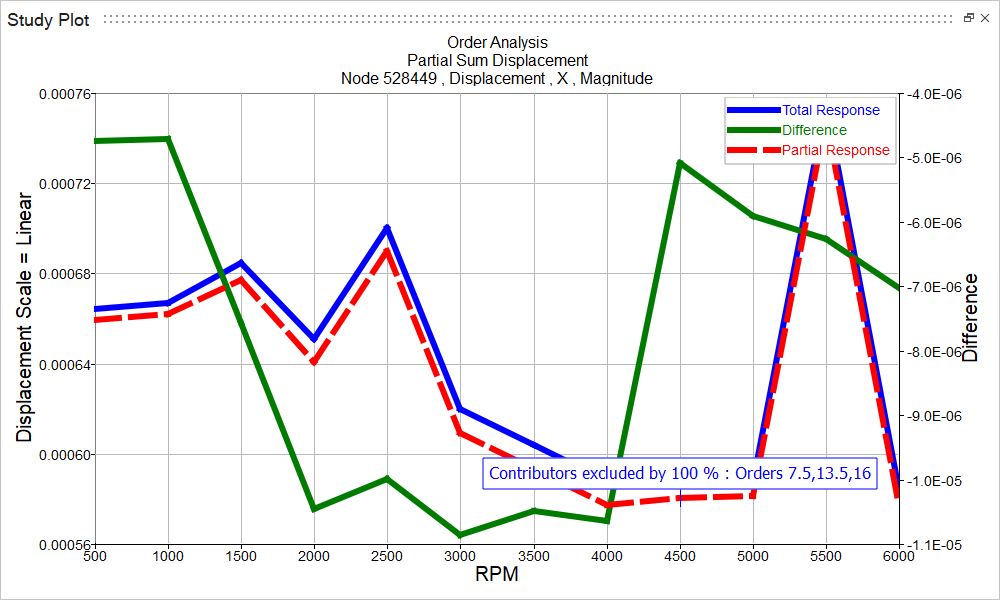
Partial sum study - Select a number of orders to exclude from the order sum response, with an optional percentage to exclude.
Order overlay - Select specific order curves to overlay with the order sum response.
% to exclude
Optional field that allows you to exclude a percentage of the orders from the order sum response.
Select order to
Select the orders that you want to exclude or include in the response study.
-
Click Select all option to select the entire list of orders.
-
Click Select all option again to deselect your current selections.
-
Click Reverse option to exchange the currently selected orders for the unselected orders in the in the list.
Show difference curve as
Shows the difference between the original curve and the partial sum curves.
To determine how the difference curve is displayed, select one of the following options from the drop-down menu:
- % of Response
- Select same as Response
Display Options
Launches the Display Options dialog, which allows you to further customize the plot.
Display
Click Display to display the response study plot once your selections are complete.
Example
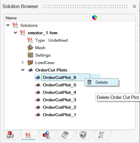
Order Plots will be listed under Solutions Tab in Model Browser for each solution.
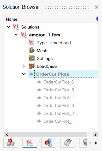
OrderCut Plots can be shown/hidden based on icon check on/off.
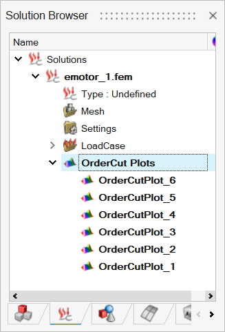
OrderCut Plots can be saved along with the database.
OrderCut Plots can be deleted using the delete option and renamed using the rename option.