Composite Topology and Free-size Optimization

For composite structures, topology and free-size optimization are defined through the DTPL and DSIZE Bulk Data Entries, respectively.

Both are supported in the HyperMesh Optimization panel. Features available include: minimum member size control, symmetry, pattern grouping and pattern repetition.

Topology and free-size methods target a system level composite design where laminate family definition is the objective. Therefore, the PCOMP model should not reflect a detailed stacking of plies of the same orientation. For example, even though 10 layers of 0 degree graphite cloth might be separated in the stacking of the final structure, the modeling for a concept study using topology and free-size should group them together in one ply in the PCOMP, so that the optimal total thickness distribution of a 0 degree ply is optimized throughout the structure.

Involving both topology and free-size in the same optimization problem is not recommended, since the penalization on topology components creates a bias that could lead to sub-optimal solutions.

Note: Prior to OptiStruct 8.0, composite topology optimization was based on the notion that the homogenized properties of an element remain unchanged. This construct does not allow the freedom for material redefinition. However, if this is indeed a preferred assumption, the HOMO option can be set on the MAT line of the DTPL card. Otherwise, an individual ply-based formulation (discussed above) will be the default option.

Problem Formulation

For a composite shell element Figure 1, the thickness ti of each ply is a variable between 0 and Ti defined on the PCOMP card.

Figure 1. Composite Shell Element

The only difference between topology and free-size here is that the former targets a discrete final solution of 0 (or Ti) for ti, while free-size allows ti to vary freely between 0 and Ti. The discrete solution is achieved by penalizing intermediate thickness. Most general characteristics of regular shell topology and free-size optimization also apply to composite. It is recommended to become familiar with Free-size Optimization before proceeding. The major differences between topology optimization and free-size can be illustrated through a simple example.

Example: Cantilever Plate

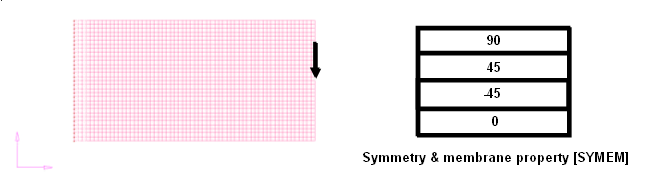
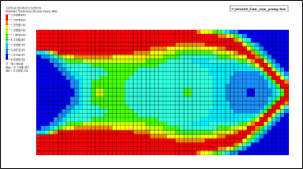
The cantilever plate shown in Figure 2. A symmetric lay-up of (0, +45, -45, and 90) degree plies are used. The optimization problem is stated as:

Minimize Compliance

Subject to Volume fraction < 0.3

For topology optimization, the thickness distribution of individual plies in the final design is shown in Figure 3.

The total thickness of the laminate is shown next.

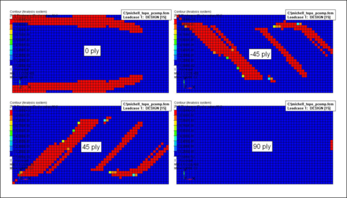
It can be seen that a rather discrete thickness for each ply is obtained. While little overlapping of different orientations is shown in this result, it should be expected that overlapping of plies of different angles might be more pronounced when multiple load cases exist.

The thickness distribution of free-size optimization for this example is shown in Figure 5.

As expected, free-size created a design in which variable ply thickness appears in a large area of the structure. The compliance of both designs are compared in Figure 7. It is not surprising to see that the free-size design outperforms the topology design in terms of compliance since a continuous variation of thickness offers more design freedom.

Figure 7. Compliance of Topology and Free-size Results

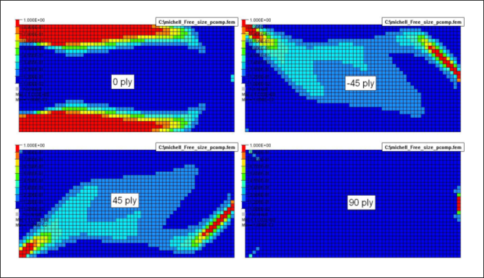
While ply angles are not variables for topology and free-size optimization, thickness optimization of plies indirectly leads to a discrete optimization of angles. The available angles in the PCOMP can be interpreted as discrete angle variables. Also, while free-size often creates variable thickness distribution without extensive cavity, it does not prevent cavity if the optimizer demands it. For this example, there is cavity in the free-size results in the 45 degree region, adjacent to the support, and in the upper and lower corners of the free end.

Topology and Free-size Design Characteristics

Most of the characteristics for general shell discussed in the free-size section also apply to composite structures.

One important exception is that the manufacturing cost is no longer a restrictive factor for composites. The reason for this is that a composite structure is manufactured by laying very thin plies of fiber cloth over each other and binding them with a matrix material, like epoxy resin. Therefore, an almost continuous change of laminate thickness can be achieved seamlessly by dropping/adding plies freely.

Table 1. Composite Topology versus Free-size Characteristics
Composite Topology	Composite Free-size
Angle optimized indirectly.	Angle optimized indirectly.
Goal - 0/Ti discrete thickness of individual plies Restricted freedom	Goal - variable thickness of individual plies "Free" under upper bound Ti
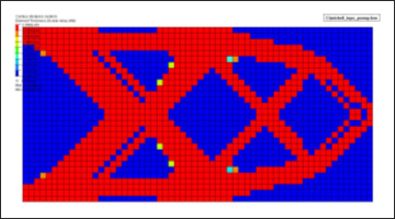
Results - Truss-like design concepts.	Variable thickness panel likely for in-plane loading, 0/1 thickness likely when bending is dominant.
Not useful compared to Free-size?	Always better design?
Manufacture - not a factor for composite unless pre-manufactured laminate is used.	Manufacture - naturally achieved with no additional cost.
Concentrated full thick members are stronger against out of plane buckling.	Spread thin shell could be prone to buckling.
Functionality may need holes for other non-structural components or for passing lines/pipes.	Cavity is controlled by optimality, and is usually not extensive under in-plane loading.

Interpret Topology and Free-size Results

Interpretation of topology results is rather straight-forward. For free-size, the change in thickness of individual plies provides insight for ply dropping/adding zones.

The thickness of each ply in each individual zone can then be defined as a design variable in a detailed size optimization. At this stage, discrete variables can be used to reflect the discrete nature of ply thickness change. Overlapping all zones of individual plies can then help to generate PCOMP zones, where a ply traveling through different zones can be defined using PCOMPG.