
Free-shape Optimization
Uses a proprietary optimization technique developed by Altair Engineering, Inc. There are two types of Free-Shape Optimization, Classic and Vertex Morphing Free-Shape.
The essential idea of free-shape optimization, and where it differs from other shape optimization techniques, is that the allowable movement of the outer boundary is automatically determined, thus relieving you of the burden of defining shape perturbations.
- Classic Free-Shape Optimization
(TYPE=CLASSIC)
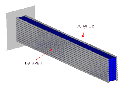
Design regions are identified by the grids on the grids are the structure (the edge of a shell structure or the surface of a solid structure). These grids are listed on the DSHAPE entry.
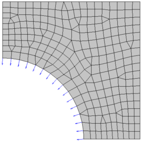
The outer boundary of a structure is altered to meet with pre-defined objectives and constraints. Allows these design grids to move in one of two ways:- For shell structures, grids move normal to the surface edge in the tangential plane.
- For solid structures, grids move normal to the surface.
During free-shape optimization, the normal directions change with the change in shape of the structure; thus, for each iteration, the design grids move along the updated normals.
- Vertex Morphing Free-Shape Optimization
(TYPE=VERTEXM)
Vertex morphing shape optimization was introduced by Dr. Bletzinger and associates. 1 In this method the vertices of all FE-mesh grids are treated as design variables. Shape smoothness is achieved by a filtering function connecting grids within a user-defined feature size radius. Compared to the CLASSIC formulation, the GRID option offers largely increased design freedom. It also overcomes the limitation in the classic free-shape formulation that only allowed in-plane shape changes of shell structures. However, computational effort of the VERTEXM method can be significantly higher, since it involves a much larger number of design variables. Adjoint sensitivity analysis is implemented for this formulation. Therefore, it is important that the user make effort to contain the number of active constraints similar to topology optimization applications.
For the Vertex Morphing free-shape optimization, the optimization design space can be defined as:- For shells – Grids in the entire design space can be selected. It does not have to only be the edge grids of the shell design domain.
- For solids – Grids should be selected on the surface of the solid
design space. Even if the internal grids are selected, then they are
ignored for the creation of design variables. Note: In the rare case wherein only internal solid grids are selected, the run will error out.
Define Free-shape Design Regions
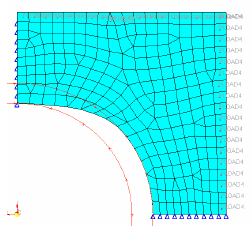
Ideally, free-shape design regions should be selected where it can be assumed that the shape of the structure is most sensitive to the concerned responses.
For example, it would be appropriate to select grids in a high stress region when the objective is to reduce stress.
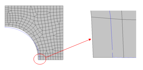
Free-shape design regions should be defined at different locations on the structure where it is desired for the shape to change independently. For solid structures, feature lines often define natural boundaries for free-shape design regions. Containing any feature lines inside a free-shape design region should be avoided unless the intention is to smooth the feature lines during an optimization. Likewise for a shell structure, sharp corners should not be contained inside a free-shape design region unless the intention is to smooth out such corners.
| (1) | (2) | (3) | (4) | (5) | (6) | (7) | (8) | (9) | (10) |
|---|---|---|---|---|---|---|---|---|---|
| GRID | GID1 | GID2 | GID3 | GID4 | GID5 | GID6 | GID7 | ||
| GID8 | GID9 | etc | etc | ||||||
Free-shape Parameters
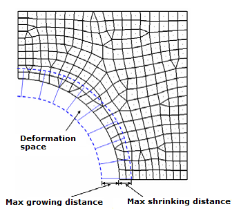
The five parameters that affect the way in which the free-shape design region deforms are the direction type, the move factor, the number of layers for mesh smoothing, the maximum shrinkage, and maximum growth.
Direction Type
| (1) | (2) | (3) | (4) | (5) | (6) | (7) | (8) | (9) | (10) |
|---|---|---|---|---|---|---|---|---|---|
| PERT | DTYPE | MVFACTOR | NSMOOTH | MXSHRK | MXGROW | SMETHOD | NTRANS |
- GROW
- Grids cannot move inside of the initial part boundary.
- SHRINK
- Grids cannot move outside of the initial part boundary.
- BOTH
- Grids are unconstrained.
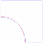

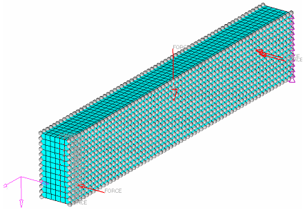
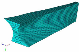
- Undeformed

- Deformed
Move Factor
MVFACTOR * mesh_size- "
mesh_size" - Average mesh size of the design region defined in the same DSHAPE card
| (1) | (2) | (3) | (4) | (5) | (6) | (7) | (8) | (9) | (10) |
|---|---|---|---|---|---|---|---|---|---|
| PERT | DTYPE | MVFACTOR | NSMOOTH | MXSHRK | MXGROW | SMETHOD | NTRANS |

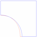
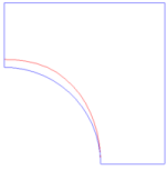
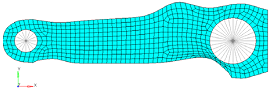
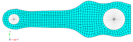
- Undeformed shape

- Shape at iteration 1 with MVFACTOR = 0.5 (default)

- Shape at iteration 1 with MVFACTOR = 1.0
Number of Layers for Mesh Smoothing
| (1) | (2) | (3) | (4) | (5) | (6) | (7) | (8) | (9) | (10) |
|---|---|---|---|---|---|---|---|---|---|
| PERT | DTYPE | MVFACTOR | NSMOOTH | MXSHRK | MXGROW | SMETHOD | NTRANS |
Maximum Shrinkage and Growth
| (1) | (2) | (3) | (4) | (5) | (6) | (7) | (8) | (9) | (10) |
|---|---|---|---|---|---|---|---|---|---|
| PERT | DTYPE | MVFACTOR | NSMOOTH | MXSHRK | MXGROW | SMETHOD | NTRANS |
For more details and an example, refer to Mesh Barrier Constraint.
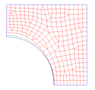
Additional Treatment to Grids in the Transition Zone
When the entire surface or edge of a system is not a design zone and both design and non-design regions exist adjacent to one another, a transition zone can be defined using NTRANS which helps to smooth out the transition. Sharp changes can occur in the design region during optimization and the sections of the design region closest to the non-design region are designated as a transition zone where the corresponding location of the adjacent non-design region is taken into consideration allowing for a smoother transition from the design to non-design region.
| (1) | (2) | (3) | (4) | (5) | (6) | (7) | (8) | (9) | (10) |
|---|---|---|---|---|---|---|---|---|---|
| PERT | DTYPE | MVFACTOR | NSMOOTH | MXSHRK | MXGROW | SMETHOD | NTRANS |
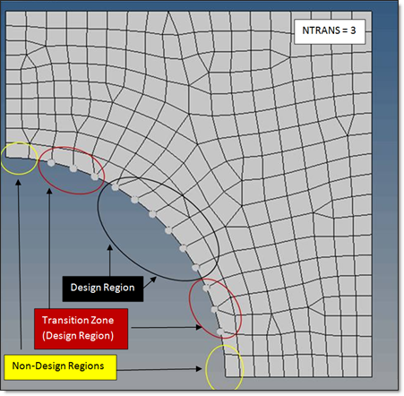
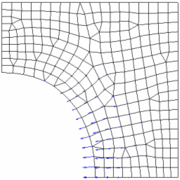
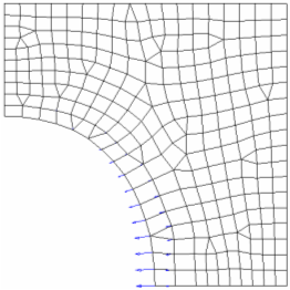
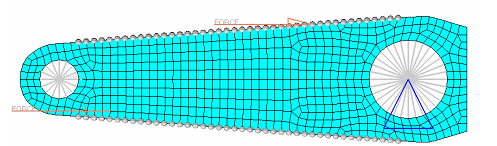
- The non-design nodes (marked by yellow circles), which do not move during Freeshape optimization.
- Design nodes in transition zone (highlighted nodes enclosed by red circles, defined by NTRANS=3)
- Design nodes that are NOT in the transition zone (highlighted nodes enclosed by a black circle)

Constraints on Grids in the Design Region
It is possible to identify additional constraints on certain grids in free-shape design regions.
- FIXED
- Grid cannot move due to free-shape optimization.
- DIR
- Grid is forced to move along the specified vector.
- NORM
- Grid is forced to remain on a plane for which the specified vector defines the normal direction.
| (1) | (2) | (3) | (4) | (5) | (6) | (7) | (8) | (9) | (10) |
|---|---|---|---|---|---|---|---|---|---|
| GRIDCON | GCMETH | GCSETID1
/ GDID1 |
CTYPE1 | CID1 | X1 | Y1 | Z1 | ||
| GCMETH | GCSETID2
/ GDID2 |
CTYPE2 | CID2 | X2 | Y2 | Z2 |
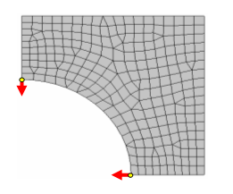
Example: CTYPE=VECTOR
This example demonstrates a simple case where it is necessary to use the "DIR" constraint type to force grids to move in a predefined direction.
Example: CTYPE=PLANAR
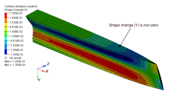
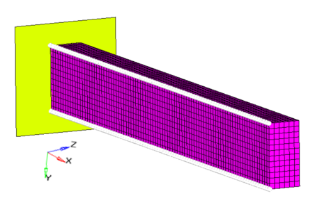
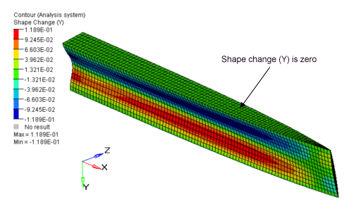
1-plane Symmetry Constraint
An advantage of this constraint is that it will produce symmetric designs regardless of the initial mesh, loads or boundary conditions.
It is often desirable to produce a symmetric design. Even if the loads and boundary conditions are perfectly symmetric, there is no guarantee that the resulting design will be perfectly symmetric. In order to ensure a symmetric design, a symmetry constraint must be defined.
| (1) | (2) | (3) | (4) | (5) | (6) | (7) | (8) | (9) | (10) |
|---|---|---|---|---|---|---|---|---|---|
| PATRN | TYP | AID/ XA |
YA | ZA | FID/ XF |
YF | ZF |
Example: 1-plane Symmetry Constraints in 2-dimensions
Example: 1-plane Symmetry Constraints in 3-dimensions
Extrusion Constraint
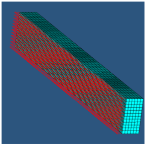
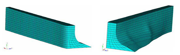
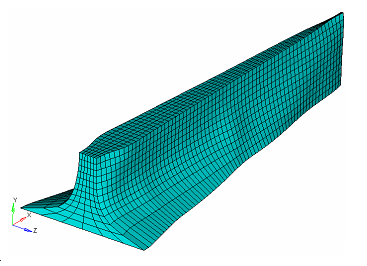
Using extrusion manufacturing constraints with free-shape optimization, constant cross-section designs can be attained for solid models (regardless of the initial mesh, loads or boundary conditions).
It is often desirable to produce a design with a constant cross-section along a given path, particularly in the case of parts manufactured by an extrusion process.
| (1) | (2) | (3) | (4) | (5) | (6) | (7) | (8) | (9) | (10) |
|---|---|---|---|---|---|---|---|---|---|
| EXTR | ECID | XE | YE | ZE |
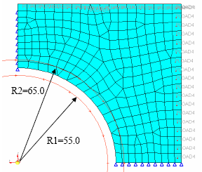
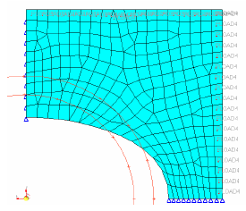
Two types of extrusion path are available for free-shape optimization - straight line and circular.
Example: Extrusion Constraint Along a Straight Line
Example: Extrusion Constraint Along a Circular Path
Draw Direction Constraint
Draw direction constraints may be defined for the design region so that the optimized shape will allow the die to slide in a specified direction.
In the casting process, cavities that are not open and lined up with the sliding direction of the die are not feasible. Only a single die is considered for each design region (defined in each DSHAPE card), and non-design regions will not be considered for this constraint.
| (1) | (2) | (3) | (4) | (5) | (6) | (7) | (8) | (9) | (10) |
|---|---|---|---|---|---|---|---|---|---|
| DRAW | DTYP | DAID/ XDA |
YDA | ZDA | DFID/ XDF |
YDF | ZDF |
Example: Draw Direction Constraint
Example: Combination of 1-plane Symmetry and Draw Direction Constraints
Side Constraints
Side constraints allow the deformation space to be defined as a coordinate range.
Similar to the maximum shrinkage and growth parameters as defined on the PERT continuation line, it is possible to limit the extent of the total deformation of the design region by way of side constraints. Side constraints allow the deformation space to be defined as a coordinate range; that is, between (x1, y1, z1) and (x2, y2, z2). These ranges may be with reference to rectangular, cylindrical or spherical systems.
Example: Side Constraints
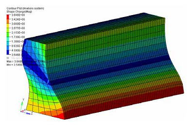
Mesh Barrier Constraints
The mesh barrier is composed of special shell elements (BMFACE), and in order to keep computational effort to a minimum, as few elements as possible should be used in its definition.
Aside from shrinkage and growth parameters and side constraints, a more general capability to limit the extent of the total deformation of the design region is available by way of defining a mesh barrier constraint.
| (1) | (2) | (3) | (4) | (5) | (6) | (7) | (8) | (9) | (10) |
|---|---|---|---|---|---|---|---|---|---|
| BMESH | BMID |
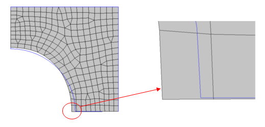
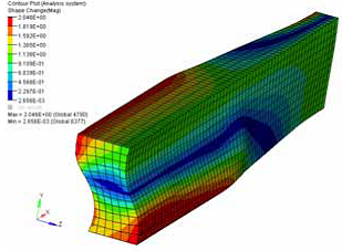
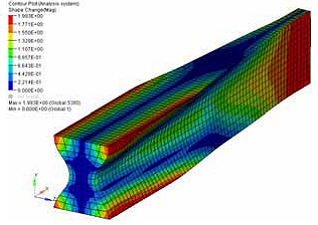
Example: Mesh Barrier Constraint
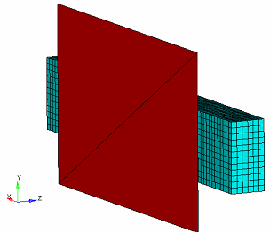
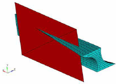
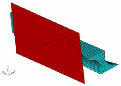
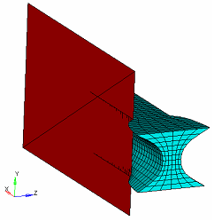
From the results, you can see how the mesh barrier constrains the model deformation, but if the mesh barrier is not big enough, the design region deformation is unconstrained beyond its limits.
Example: Maximum Shrinkage and Growth Parameters
Comments
- When multiple constraints are defined for the same design region, while the optimizer tries its best to satisfy all the different constraints, it is possible that it may not be able to coordinate all these constraints.
- It should be pointed out that if constraints like mesh barrier, maximum growth and shrinkage, or side constraints are applied to avoid of interference between structural parts, the constraints should be defined in such a way that clearance is guaranteed under manufacturing tolerance and structural deformation. In other words, the barrier surface should contain an offset from the potentially interfering parts.