
Equivalent Static Load Method (ESLM)
A technique suitable for optimization of designs undergoing dynamic loads.
- Multibody dynamics problems including flexible bodies
- Nonlinear responses from implicit static analysis, implicit dynamic analysis and explicit dynamic analysis
The equivalent static load method takes advantage of the well established static response optimization capabilities of OptiStruct.
Equivalent Static Load

The equivalent static load is that load which creates the same response field as that of the dynamic/nonlinear analysis at a given time step. From Figure 1, an equivalent static load is calculated corresponding to each time step in the time history of the solution, thereby replicating the dynamic/nonlinear behavior of the system in a static environment.

The equivalent static load method is completely automated in OptiStruct and is an efficient approach for the optimization of responses from transient, dynamic and nonlinear solutions.
- It can be applied at the concept design phase as well as design fine tuning phase, that is, it can be used with topology, free-sizing, topography, size, shape and free-shape optimization.
- A design is optimized for updated loads, due to an updated design during the optimization process.
ESL Optimization Convergence Criteria
- There is no change in both the objective function value and in the maximum constraint violation between two outer loops.
- There is no improvement in both the objective and in the maximum constraint violation between to outer loops.
- The previous six objective function values oscillated around the optimum.
ESLM for MBD
The equivalent static load method has been implemented for the solution of multibody dynamics problems that include flexible bodies.
Size, shape, free-shape, topology, topography, free-size, and material optimization can be applied to flexible bodies. Responses are mass, volume, center of gravity, moment of inertia, stress, strain, compliance (strain energy), and displacement of the flexible bodies. Displacement responses are taken into account with respect to local boundary conditions defined on the flexible body (see definition below). Responses are defined using DRESP1, DRESP2, and DRESP3 Bulk Data Entries. Responses can only be defined on flexible bodies (PFBODY) using the properties, elements and grid points included in such bodies as reference. Design variables are defined using DESVAR, DVPREL1, DVPREL2, DVMREL1, DVMREL2, DSHAPE, DTPL, DTPG, DSIZE, and DVGRID Bulk Data Entries. Free-size optimization is currently only available when PTYPE=PSHELL on the DSIZE card. Design variables can only be defined on flexible bodies (PFBODY) using the properties included in such bodies as reference. Constraints are defined using DCONSTR, DCONADD and DOBJREF Bulk Data Entries. Constraints and objectives are referenced in the multibody dynamics subcase or globally through DESOBJ, DESSUB, DESGLB, and MINMAX, respectively.
ESLM specific parameters can be set through the DOPTPRM Bulk Data Entry (Parameters).
Method
An optimum solution can be found through a series of static response optimizations with the equivalent static load set, that is:
- Equivalent static load
- Deformation
- Acceleration
- Velocity
- External load
- Step 1
- Initial design.
- Step 2
- Dynamic analysis.
- Step 3
- Static response optimization with the multiple subcases that consist of multiple equivalent static load sets.
- Step 4
- If design converged, Stop. Otherwise go to Step 2.
The iteration at the third step is referred to as an inner iteration; Steps 2 through 4 form the outer loop. The converged solution at Step 3 is the starting point of the next outer loop (if the design does not converge at the current outer loop). If there are time steps in the multibody dynamics analysis at Step 2, subcases in static response optimization are generated at Step 3 (provided that the time step screening option is deactivated). See Parameters.
Boundary Conditions for Structural Analysis and Optimization
To perform structural optimization with ESL, you must specify boundary conditions for each flexible body. In the solution of the dynamic analysis, the flexible and rigid bodies are connected by joints to form a multibody system.
When performing ESLM on the flexible bodies, these joints are not included in this static subcase-based structural optimization. This means that each flexible body will have 6 rigid body modes. The 6 rigid body modes of each flexible body must be removed for structural analysis. Exactly 6 degrees of freedom (DOF) of each flexible body must be fixed to remove the 6 rigid body modes. If more than 6 DOF are fixed in a flexible body, the additional fixed DOF become the constraint of the flexible body, which may not result in an optimal solution and consequently increases the required ESLM outer loops.
Due to the way ESL is calculated, each flexible body is in its equilibrium at the 0-th inner iteration of each outer loop. This is why you can fix an arbitrary 6DOF (usually single node) to get rid of rigid body modes in order to do static analysis with ESL. Reaction force at the fixed node is zero at the 0-th inner iteration. Thus, no additional load is applied to a flexible body although 6 DOF of the flexible body are fixed. However, design changes occur as the inner iteration goes on. This means the original configuration that maintains equilibrium also changes. As a result, the equilibrium status does not hold true anymore from the 1st inner iteration in each outer loop. An undesirable effect caused by a broken equilibrium status (disequilibrium status) is the reaction force at the fixed point is not zero anymore, which means additional load is applied to that fixed point. This effect, due to shape/size changes, can be minimized by fixing a proper node, as explained below.
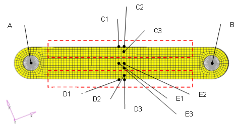
Nodes A and B are the locations of joints. The best option here is to fix 6 DOF of either node (A or B) in order to remove 6 rigid body motions in this model. To fix alternative nodes other than node A or B, it would work to fix 3 DOF (123) of node E1, 2 DOF (23) of node E2, and 1 DOF (3) of node E3. These three nodes are located in a relatively low stress region. In this model, nodes C1, C2, and C3 or nodes D1, D2, and D3 would take a long time to converge if fixed. Again, the best and simplest way to remove 6 rigid body modes of each flexible body is to fix one of the joint locations in each flexible body.


Output Files Generated by the Optimization Process
Output files are generated after ESL optimization converges.
- .eslout
- This text file contains brief and useful information about the
optimization process. Open this file first to find out what occurred
during the ESL optimization. This file is often enough to understand the
overall optimization process. The following information is stored in
this file:
- Involved time steps and corresponding subcases
- The number of involved time steps
- Design results
- The number of inner iterations
- CPU time
- _mbd_#.h3d
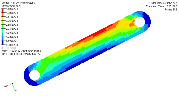
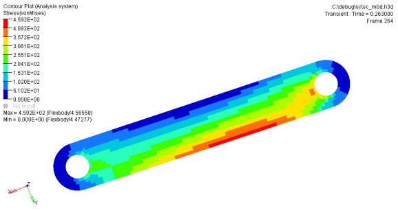
- This binary output file contains the MBD analysis results of the #-th outer loop. Displacement, stress, and deformation are available in this file. This file is a modal H3D format (PARAM,MBDH3D,MODAL), which is only available format in ESL optimization. HyperView can display this file.
- _des_#.h3d
- This binary output file contains design change of the #-th outer loop. By selecting the contour button, you can see the design change. HyperView can display this file.
- _mbd_#.abf
- This binary output file contains information about rigid body dynamics and modal participation factors of the #-th outer loop. HyperGraph can display the data stored in this file.
In addition to the above output files, .desvar, .prop, .grid, .fsthick, and .oss will be found, if available.
Convergence Enhancement
It is important to catch the critical responses of a structure properly when optimizing the structure. Generally, it is a good practice to define many time steps in the time intervals where the critical responses of interest show up.
By doing this, the optimizer can consider more precise responses at the critical time intervals, resulting in a decreased probability that the optimizer will go in the wrong direction in the current outer loop.
MBSIM 4 TRANS END 1.0 NSTEPS 100$more time steps from 0.0 sec to 0.02 sec.
MBSIM 1 TRANS END 0.02 NSTEPS 200
+ VSTIFF
MBSIM 2 TRANS END 0.61 NSTEPS 200
+ VSTIFF
$more time steps from 0.61 sec to 0.63 sec.
MBSIM 3 TRANS END 0.63 NSTEPS 200
+ VSTIFF
MBSIM 4 TRANS END 1.0 NSTEPS 100
$
MBSEQ 10 1 2 3 4
In the above MBSIM cards, time steps in the time interval 0 to 0.02 seconds and the time interval 0.61 and 0.63 seconds have been increased. Generally, the more information the optimizer is provided, the better the solution it can provide. It is beneficial to define many time steps; enough to catch precisely the critical responses in the time intervals where critical response of interest show up. This will enhance convergence of the optimization process.
Parameters
Control the maximum number of outer loops executed in ESLM.
DOPTPRM, ESLMAXIn this case, the ESLMAX is an integer value, greater than or equal to 0. If the ESLMAX is equal to 0, the optimization process is not activated. The default value for the ESLMAX is 30.
DOPTPRM, ESLSOPTThe ESLSOPT can be either 0 or 1. If ESLSOPT is 0, the screening is deactivated. If ESLSOPT is 1, this screening is activated. The default value is 1. Unless deactivated by DOPTPRM,ESLSOPT,0, this feature is always activated.
The time step screening feature is different from the constraint screening of the static response optimization in Step 3, although the concepts of both screening capabilities are similar. The time step screening is performed at time Step 2, which is right before entering the static response optimization phase. By performing the time step screening before entering the static response optimization phase, the huge amounts of CPU time required for structural analysis and subsequent constraint screening strategy can be saved at the 0-th iteration in the static response optimization phase.
DOPTPRM, ESLSTOLESLSTOL is a real number between 0.0 and 1.0. The smaller the value of ESLSTOL, the fewer the number of time steps involved in the optimization process. If ESLSTOL is 1.0, all of the time steps in multibody dynamic analysis will be involved in the optimization process. Obviously, the smaller the ESLSTOL value, the less total CPU time will be used. Note, however, that assigning too small a value to the ESLSTOL could cause the optimization process to diverge. Therefore, if the number of time steps retained by ESLSTOL is less than 10, the 10 most dominant time steps will be involved in the optimization process. The default value for the ESLSTOL is 0.3.
Output Requests
Users are not allowed to control analysis output in ESL optimization. All information from the MBD analysis is already available in _mbd_#.h3d, including displacement, stress, and deformation.
All analysis output requests are invalidated during ESL optimization except that Output Request = option is allowed above the first subcase. For example, STRESS=ALL or DISPLACEMENT=SID is allowed above the first subcase.
Optimization output is not controllable in ESL optimization. See Equivalent Static Load Method (ESLM) for more details.
Output and format in output format controls are not controllable in ESL optimization. All requests on output and format are invalidated during ESL optimization, except for FSTHICK and OSS.
MBD System Level Response Optimization
The original ESLM implemented in OptiStruct is for the optimization of flexible bodies in MBD systems through the control of structural responses, such as stress or deformation.
Minimize joint force of a joint
subject to stress < allowable value
deformation < allowable value
velocities of a node < allowable value
MBD system level responses can be controlled by the properties of PRBODY, CMBUSH(M), CMBEAM(M), and CMSPDP(M) as well as usual design variables in structural optimization such as thickness of bodies, shape of bodies, etc. DVMBRL1 and DVMBRL2 are available to define relationships between design variables and properties of PRBODY, CMBUSH(M), CMBEAM(M), and CMSPDP(M).
Large Number of Design Variables
MBD system level responses are approximated by adaptive response surfaces.
The basic solution strategy for MBD system level optimization is the same as that implemented in HyperStudy. In general, response surface-based optimization cannot handle large number of design variables. This issue has been resolved in OptiStruct through the introduction of intermediate design variables for bodies. All the design variables defined on rigid/flexible bodies are converted to some predefined intermediate design variables. Adaptive response surfaces are built based on those intermediate design variables. As a result, even if there are hundreds of design variables defined on bodies, adaptive response surfaces for MBD system level responses can be built with only several intermediate design variables. This way, OptiStruct can handle MBD system level responses with large number of design variables.
Change Length of Bodies as Shape Optimization
When you try to achieve a specific velocity value less than an allowed value, changing the length of bodies is an efficient way to achieve it. You can set up a shape optimization problem to change the length of bodies.
The designable bodies can be either rigid bodies or flexible bodies. When defining shape perturbation vectors with DVGRID, make sure that each perturbation vector does not break down the original joint configuration as the design changes. For example, a revolute joint must have two coincident nodes attached to two different bodies. Be aware while defining shape perturbation vectors, that the perturbation vector could cause a location change for only one of the two coincident nodes so that the revolute joint definition would not be valid after one design iteration.
Limitations
Design variables associated with PRBODY, CMBUSH(M), CMBEAM(M), and CMSPDP(M) cannot control structural responses, such as deformation or stress.
They can only control MBD system level responses such as MBDIS, MBVEL, MBACC, MBFRC, and MBEXPR. Design variables associated with structures such as length, shape, and thickness can control MBD system level responses. Thus, if interaction between structural responses and MBD system level responses are mutually strong, this feature is not applicable.
Rigid bodies cannot have structural design variables (shape, properties, thickness, etc.) and the design variables associated with DVMBRL1/DVMBRL2 with TYPE=PRBODY at the same time.
Currently, system level responses must be scalar values. OptiStruct provides an option to pick up the maximum, minimum, maximum absolute, or minimum absolute value of displacement/velocity/acceleration/joint force when defining MBD system level responses using the DRESP1 card. If a system level response is an objective function, and the time when the objective function is picked up jumps around during the optimization process, convergence could be slow or even diverge in some cases.