Lattice Structure Optimization

A novel solution to create blended Solid and Lattice structures from concept to detailed final design.

This technology is developed in particular to assist design innovation for additive layer manufacturing (3D printing). The solution is achieved through two optimization phases. Phase I carries out classic Topology Optimization, albeit reduced penalty options are provided to allow more porous material with intermediate density to exist. Phase 2 transforms porous zones from Phase 1 into explicit lattice structure. Then lattice member dimensions are optimized in the second phase, typically with detailed constraints on stress, displacements, etc. The final result is a structure blended with solid parts and lattice zones of varying material volume. For this release two types of lattice cell layout are offered: tetrahedron and pyramid/diamond cells derived from tetrahedral and hexahedral meshes, respectively. For this release the lattice cell size is directly related to the mesh size in the model.

Motivation

Lattice Structure Optimization is initially similar to topology optimization; however, design domains can now include elements with intermediate densities. Theoretically, from a physical point of view, such structures can be more efficient compared to those in which design elements are penalized to densities of 0 or 1.

Figure 1. Difference between Lattice Optimization (Phase 1) and Topology Optimization

A possible major application of Lattice Structure Optimization is Additive Layer Manufacturing which can take advantage of the intricate lattice representation of the intermediate densities. This can lead to more efficient structures as compared to blocky structures, which require more material to sustain similar loading.

It should be noted that typically porous material represented by periodic lattice structures exhibits lower stiffness per volume unit compared to fully dense material. For tetrahedron and diamond lattice cells, the homogenized Young's modulus to density relationship is approximately given as $E = ρ^{1.8} E_{0}$ , where $E_{0}$ specifies Young's modulus of the dense material. Varying levels of lattice/porous domains in topology results are controlled by the parameter POROSITY. With POROSITY defined as LOW, the natural penalty of 1.8 is applied, which would typically lead to a final design with mostly fully dense materials distribution (or voids) if a simple 'stiffest structure' formulation (compliance minimization for a given target volume) is applied. However, you may favor higher proportion of lattice zones in the design for considerations other than stiffness. These can include considerations for buckling behavior, thermal performance, dynamic characteristics, and so on. Also, for applications such as biomedical implants porosity of the component can be an important functional requirement. For such requirements, there are two different options for POROSITY. At HIGH, no penalty is applied to Young's modulus to density relationship, typically resulting in a high portion of lattice zones in the final results of Phase I. At MED, a reduced penalty of 1.25 is applied for a medium level of preference for lattice presence.

Design constraints can be defined in both Phase 1 and 2 of the Lattice Optimization process. Some specific constraints, like stresses (via LATSTR) are not applied to the first phase, but passed to the second phase. Although some design constraints are applied during Phase 1, it is important to consider every required design constraint during Phase 2 of the optimization process. The design constraints defined in Phase 2 should be sufficiently exhaustive to sustain the use case if the final design is expected to be '3D printed' directly. For traditional structures, users usually go through a second stage where the topology concept is interpreted and then fine-tuned by size optimization with all design constraints included. The second phase of the lattice optimization process should be viewed as the fine-tuning stage for the design since further manual manipulation of a lattice structure with hundreds of thousands cell members is close to impossible.

Note: During Phase 2, Euler Buckling constraints are automatically applied to the Lattice Structure model. In theory, the column effective length factor in the Euler buckling calculation for the lattice beams, varies depending on the boundary conditions affecting a particular beam. The main boundary condition influencing the column effective length factor is the way the beam is attached at its ends. Typically, the factor varies from ideally hinged (1.0) to rigidly fixed (0.5). In OptiStruct, the column effective length factor is internally set equal to a value between the two. This value is set equal to the same value for all beams. Therefore, this implies that the resulting structure will be less conservative as compared to an ideally hinged model. If buckling performance is critical to the model, then you need to make sure the performance of the final structure is as expected. Additionally, the Buckling Safety Factor (LATPRM, BUCKSF) can be used to adjust the safety factor of the buckling load calculation. If you reset the internally created parameter LATPRM, LATTICE, YES is reset to NO, the Euler Buckling constraints are deactivated (not recommended).

Restriction:

Global-Local Analysis and Multi-Model Optimization are currently not supported in Lattice Optimization.
Shape, Free-size, Equivalent Static Load (ESL), Topography, and Level-set Topology optimizations are not supported in conjunction with Lattice Optimization.
Heat-Transfer Analysis and Fluid-Structure Interaction are not supported.

Lattice Generation (Phase 1)

In the first phase, the design domains are optimized similar to a regular topology optimization, except that intermediate density elements are retained in the model.

As explained above, this theoretically may improve performance of the optimized structure for considerations other than compliance (for example, buckling) when compared to a regular topology optimization. The intermediate densities in the optimized structure are represented by user-defined lattice types (micro-structures). The volume fraction of the lattice structure corresponds to the element density at the end of the first phase. During the optimization process, stiffness of the intermediate densities corresponds to micro-structural homogenized properties.

Definition

The first phase of the Lattice optimization process requires the inclusion of the LATTICE continuation line on all DTPL Bulk Data Entries. This activates Lattice optimization, and the LB and UB fields can be used to specify the range of densities for elements that can be converted into Lattice elements. Elements with densities above UB remain as solid elements and those with densities lower than LB are removed from the model.

The solid elements which lie within the LB and UB density bounds (intermediate densities) defined on the LATTICE continuation line are replaced by the corresponding Lattice Structures (Lattice Type - LT). The solid elements can be first or second order elements. The lattice structures are constructed using 1D Tapered Beam (CBEAM) elements (Figure 2). The initial radius of the lattice structure beam elements for each lattice structure cell is proportional to the density of the intermediate density elements which were replaced, such that the initial volume in phase 2 is equal to that at the end of phase 1. In phase 2, the concept of lattice beam element radius is interpreted as joint thickness. Thickness for each joint at the conjunction of lattice beam elements is determined and the radius of each element can vary across the beam length. The beam elements have the property PBEAML and TYPE=ROD is automatically assigned for each element. The thickness of this tapered beam element can vary along its length and only circular cross-sections are available. The X(1)/XB field on the PBEAML entry is always set to 1.0 for tapered beam elements.

For TYPE=ROD, if X(1)/XB is equal to 1.0, the DIM(1)A references the radius of the beam at end A and DIM(1)1 references the radius of the beam at end B. This element is a tapered beam formulation, and averaging is not used to determine the average radius of the beam. Instead, the true tapered beam formulation is used with the given dimensions. The true tapered beam formulation is only available for TYPE=ROD.

Figure 2. Tapered Beam Formulation

The LATSTR field on the LATTICE continuation line can be used to specify the stress constraint for the second phase (Stress Constraints).

The lattice type can be controlled using the LT field on the LATTICE continuation line. This field only applies to hexahedral elements, as the other element types only have a single lattice type associated with them. For hexahedral elements, the values LT = 1, 2, 3, or 4 can be used to control the Lattice structure which replaces the intermediate density elements.

Note: The LT field is only applicable to hexahedral elements.

Lattice Types

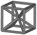
LT = 1

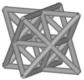
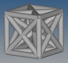
LT = 2: For LT=2, CHEXA elements, the floating grid points at the center of lattice structure faces facing the adjacent solid element at the Lattice-Solid Interface are connected using automatically generated Freeze CONTACT. The automatic creation of such CONTACT is to make certain that the center nodes on the faces connected to the solid elements are not left floating (disconnected) in the second phase.

LT = 3

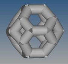
LT = 4

Note:

The lattice is based on newly created nodes only. Therefore, SPC's and FORCE's that existed in the original model and were applied to design domain will not be preserved and you will have to redefine them.
Contact interfaces with a minimum of one surface in the design domain will also not be preserved. OptiStruct internally creates new N2S contacts between the new nodes and solid elements. It is recommended to verify the newly generated contact interfaces to make certain the contact behavior is as expected.

Tetrahedral elements (CTETRA)
Pyramid elements (CPYRA)
Pentahedron elements (CPENTA)

If a Lattice Optimization solver deck is named <name>.fem, then at the end of the first phase a new file <name>_lattice.fem is generated. This new file includes the 1D element data which represents the new Lattice Structure and the sizing optimization set-up. You have to redefine optimization responses, constraints, and the objective function; additionally the contact sets may also have to be redefined (Contact).

Porosity Control

The amount of intermediate densities in a model depends primarily on the penalty applied. This is similar to the penalty applied during a topology optimization. If the penalty is increased, the intermediate densities are pushed more towards either 0.0 or 1.0. This leads to a low number of elements with intermediate densities, which corresponds to a lower percentage of lattice structures (low porosity). If the penalty is reduced, the percentage of lattice structures, are higher (high porosity).

The design parameter LATPRM, POROSITY can be used to control the porosity of the model by controlling the amount of intermediate densities in the model in the first stage of the Lattice Structure Optimization run (default = HIGH).

HIGH: This option generates a relatively high number of intermediate density elements in the first stage of the optimization run (high porosity). If this option is selected, no penalty is applied to the Young's modulus to density relationship. This generally results in a high volume fraction of lattice zones in the final results of Phase 1.
Note: This possibly leads to an over-estimation of stiffness performance for a particular model. This implies that the stiffness performance can drop significantly in Phase 2.
MED: This option generates a relatively medium number of intermediate density elements in the first stage of the optimization run (medium porosity). If this option is selected, a reduced penalty of 1.25 is applied for a medium level of preference for lattice zone presence. Typically, this option leads to a reduced number of Lattice zones as compared to the option HIGH.
LOW: This option generates a relatively low number of intermediate density elements in the first stage of the optimization run (low porosity). If this option is selected, a natural penalty of 1.8 is applied, which would typically lead to a final design with mostly fully dense material distribution if a simple "stiffest structure" formulation (compliance minimization for a given target volume) is applied.

Figure 3. Difference Between HIGH, MED, and LOW Porosity Options

Stiffness Penalization

During Phase 1, a modified topology optimization is carried out to generate a structure with a range of intermediate densities (0.0 to 1.0).

The density of a topology element is correlated to its stiffness using:(1)

E = E_{0} ρ^{p}

Where,

$E$: Optimum stiffness of the topology element for the density $ρ$
$E_{0}$: Stiffness of the initial design space material (actual material data)
$ρ$: Density (or volume fraction) of a topology element
$P$: Penalty applied to the density to control the generation of intermediate density elements

In the real world, there is no physical material that can be used for elements with "intermediate densities" since this is a virtual concept. However, with the availability of Lattice Structures, you can approximate the behavior of these virtual "intermediate densities" using varying volume fractions (or densities) and types of interconnected Beam (CBEAM) elements for each topology element. However, based on the nature of these Lattice elements, they provide a reasonably accurate physical representation of the intermediate densities only when the volume fraction to stiffness relationship is:(2)

E = ρ^{1.8} E_{0}

This is calculated by homogenizing the lattice structure within its unit volume and comparing its stiffness with the density-penalized stiffness of the modified topology optimization. Based on extensive testing, it has been observed that an optimized topology design cell is accurately represented by a lattice unit cell if the penalty is set to 1.8 in the initial modified topology optimization.

In other words, the accuracy of the correlation between the physical lattice structures and virtual intermediate densities increases as it gets closer to a penalty ( $ρ$ ) of 1.8. This is called a natural penalty and corresponds to POROSITY=LOW.

However, in some cases, a more porous structure for considerations other than compliance performance may be required (for example buckling). Then, POROSITY=MED or HIGH can be used to set lower penalty (p) values leading to a higher number of virtual intermediate elements. The number of intermediate elements is typically highest in the case of HIGH (

ρ

=1.0 or no penalty) and lower in the case of MED (

ρ

=1.25). These intermediate density elements will be replaced with lattice structures which correlate to a higher compliance (as explained earlier, the best compliance performance is only achieved when the penalty is close to 1.8). Therefore, when MED or HIGH porosity options are used, it is important to make certain that all the critical constraints are included in Phase 2 as the structural and optimization responses may be overestimated (the difference is more pronounced when HIGH is used). Moreover, it is recommended to include these critical constraints in Phase 1 also; however, with possibly more conservative bounds when compared to Phase 2. The analysis of the <name>_lattice.fem file, which is generated at the end of Phase 1, provides a more accurate picture of the compliance performance as it contains the actual Lattice structures, instead of the virtual intermediate density elements (Figure 4).

Figure 4. Difference Between LOW, MED, and HIGH Porosity Options with Regard to Stiffness Performance

If Phase 1 constraints are important, then it is recommended to choose one or more of the following:

The constraints on the original topology design space should be stricter (or tighter) than required, so as to compensate for the typical loss of stiffness after the intermediate density elements are replaced by the lattice structures (MED and HIGH porosity options).
Use POROSITY=LOW to align the modified topology optimization of the initial design space to the natural "homogenized" penalty value of the lattice structures (1.8). This results in a reasonably close approximation of the optimized design space that is replaced with lattice structures.

Size (Parameter) Optimization (Phase 2)

In the second phase, the Lattice Structure is optimized using Size optimization.

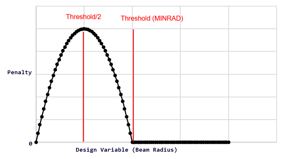
The first phase represents isotropic material optimization since the Lattice micro-structural representation has isotropic (or near-isotropic) homogenized properties. The size (parameter) optimization phase is aimed at incorporating some anisotropy to the Lattice Structure, thereby making the structure more efficient. For a given loading, the newly created file <name>_lattice.fem includes sizing (parameter) optimization set-up. The optimization responses, constraints, and objective function should be reviewed and redefined (if necessary) in the second phase. The contact sets should also be reviewed and possibly redefined if required. A single design variable (DESVAR) is automatically created for each joint (conjunction of lattice tapered beam elements) representing the radius of all the beam cross sections at the joint. The DESVAR's are related to the radii of each tapered beam element by DVPREL entries in the size (parameter) optimization process. The lower bound of the sizing design variables are automatically set to a very low value (equal to $(U B / 10^{6})$ ).

Where, UB is the upper bound of the design variables for Lattice Sizing (Parameter) Optimization phase. This lower bound can be controlled using LATPRM,MINRAD and LATPRM,CLEAN (refer to Lattice Sizing+ for more information).

At the end of the second phase, a new <name>_lattice_optimized.fem file is created, which includes optimized lattice structures. Beams with very small radii are automatically removed from the structure during this phase (Lattice Sizing+). Therefore, a verification analysis using the <name>_lattice_optimized.fem file is recommended to look at the final responses.

The parameter LATPRM,TETSPLT,YES can be used to turn on the splitting of all non-design or solid elements to Tetrahedral elements for further usage in 3D printing software.

Compliance Management

During the phases of the Lattice Optimization run, the compliance of the model varies based on different internal processes.

Reduction in compliance is generally undesirable and it is necessary to exercise caution and be aware of stages when performance drops occur.

Performance loss occurs at the end of Phase 1, due to the removal of voids and low density elements in the model (elements with a density below LB are removed). LATPRM, LATLB can be used to verify if the chosen LB value leads to a large drop in compliance.
An additional drop in performance occurs during the transition from Phase 1 to Phase 2, wherein, the intermediate density elements are replaced with corresponding Lattice Structures. If no penalty (POROSITY, HIGH) or low penalty (POROSITY, MED) is applied to the model, then after intermediate density elements are replaced by lattices, the stiffness of the structure is overestimated.

Stress Constraints

In addition to the regular constraints, stress constraints can be used in lattice optimization. Stress constraints can be applied in two ways:

The LATSTR field on the LATTICE continuation line in the DTPL entry can be used to define the stress constraint for the second phase. The stress constraint method can be selected using LATPRM, STRMETH. The stress upper bound value (LATSTR) is not applied for the first phase; instead, it is passed through to the second phase. For the CBEAM elements in the second phase corresponding DRESP1 response(s) is (are) created based on the defined stress constraint. If LATPRM, STRMETH, PNORM (default) is specified, the Stress NORM method is used to calculate the maximum stress value that is constrained for a given set of CBEAM elements. It is important to use the Stress NORM for stress constraints in the second phase due to the large number of beam elements. If stress constraints for all beams are considered as individual constraints in the optimization problem, the size of the optimization problem would be too large. The application of Stress NORM in the second phase, Euler buckling constraints, and the Lattice Sizing+ process are controlled by the internally generated parameter LATPRM, LATTICE, YES. Further modification of this parameter is not recommended. If this parameter is reset to NO, the stress NORM method is not applied in the handling of stress constraints in the second phase. This can possibly lead to a slow optimization run or maybe even termination of the program with an "Optimization problem is too large" error. The usage of Stress NORM improves efficiency of the handling of stress constraints in the second phase so it is recommended to retain the LATTICE parameter set to YES (Additionally, the LATPRM, LATTICE, YES parameter activates Euler Buckling constraints in phase 2). The Stress NORM feature creates two responses for a model, one stress NORM response for the elements with highest 10% of the stresses and a second stress NORM response for the rest of the model. Therefore, there may be two Stress Responses in the Retained Responses table of the OUT file.
The STRESS field on the DTPL entry can be used to specify stress constraints for the first phase topology optimization. This stress constraint is not passed through to the second phase.
DRESP1 stress responses are not allowed in the first phase (topology) of the lattice optimization.
Stress NORM Method

The Stress NORM method is used to approximately calculate the maximum value of the stresses of all the elements included in a particular response. This is also scaled with the stress bounds specified for each element. Therefore, to minimize the maximum stresses in a particular element set, the resulting stress NORM value ( $σ_{N O R M}$ ) is internally constrained to a value lower than 1.0.(3) $σ_{N O R M} = {(\frac{1}{n} \sum_{i = 1}^{n} {(\frac{σ_{i}}{σ_{b o u n d}})}^{p})}^{\frac{1}{p}}$

Where,

$σ_{N O R M}$

Stress NORM value

$n$

Number of elements

$σ_{i}$

Individual stress value of each element $i$

$σ_{b o u n d}$

Stress bound for each element

$p$

Penalty (power) value (default = 6.0)

The Penalty or Power value ( $p$ ) can be modified using the parameter DOPTPRM, PNORM.

The value $p$ = 6.0 is the default and higher values of ( $p$ → $\infty$ ) increases the accuracy of the stress norm function ( $σ_{N O R M}$ → $(\frac{σ_{\max}}{σ_{b o u n d}})$ ), which can lead to instability of the optimization run. Values lower than 6 ( $p$ → 1) moves the stress norm function closer to the average ratio ( $σ_{N O R M}$ → $\frac{1}{n} \sum_{i = 1}^{n} (\frac{σ_{i}}{σ_{b o u n d}})$ ). The default value is a reasonable approximation of the maximum ratio value and reduces instability.

The Stress NORM feature creates two responses for a model, one stress NORM response for the elements with highest 10% of the stresses and a second stress NORM response for the rest of the model. Therefore, there may be two Stress Responses in the Retained Responses table of the OUT file.
In addition to the default Stress Norm method, an alternative method can be selected using LATPRM,STRMETH,FSD. The alternative method may be faster for some models.

Contact

Typically, two types of CONTACT situations occur in Lattice Optimization Structures:

As described in the Lattice Type 2 section, for CHEXA elements (LT=2), Lattice structures at the design-non design interface are connected to the non-design solid elements at the corner face nodes. However, in LT=2, floating grid points are present at the face centers of the lattice structure faces adjacent to the non-design solid elements at the interface. These floating grid points are connected using automatically generated Freeze CONTACT's. If the CONTACT's are not created, the center node on the faces connected to the solid elements, are left hanging in the second phase.
The second CONTACT scenario occurs when the model contains preexisting contacts before Phase 1 is run. In such cases, prior to running Phase 2, it is recommended to review and update the contact interface, between the design, non-design, and newly created lattice domains. The Lattice domain is always set as Secondary and the non-design/solid domain in contact with the lattices is set as the Main. If this is not the case, then OptiStruct will automatically reset them to the correct order. OptiStruct will also convert S2S contact to N2S contact for lattice domains in contact with non-design domains. Additionally, in such cases, GRID sets are not allowed for defining the non-design Main (Surfaces or Element sets should be used).

Lattice Sizing+

Lattice Sizing+ is an extended sizing optimization process at the end of the sizing optimization during the second phase of lattice optimization.

Lattice Sizing+ is activated when LATPRM,CLEAN,YES (default) or LATPRM,CLEAN,LESS is present in the model. The Beam Cleaning procedure occurs after sizing optimization at the end of the second optimization phase to penalize beams with very low radii (below LATPRM,MINRAD). The beams below MINRAD are pushed to 0 or 1 via an embedded Topology optimization. The minimum value of the radii or aspect ratio can be controlled using LATPRM, MINRAD and/or LATPRM, R2LRATIO in conjunction with LATPRM, CLEAN.

The embedded topology optimization consists of two additional phases at the end of the sizing optimization phase. The first additional phase involves adding the following penalty term to the objective. This is equivalent to adding a value equal to the objective at convergence of the sizing optimization to the objective.(4)

p e n = (\sum_{i = 1}^{n_{D V}} p e n_{i}) \frac{o b j_{c}}{p e n_{c}}

Where,

$p e n$: Penalty term added to the objective
$p e n_{i}$: Penalty value associated with each sizing design variable
$o b j_{c}$: Objective value at the convergence of the previous sizing optimization phase
$p e n_{c}$: Value of the total penalty at the end of the previous sizing optimization phase

The penalty value for each design variable (beam radius) is calculated based on the chosen method on LATPRM,CLEAN. If YES is selected, then the Heaviside penalty function is used, and the Quadratic penalty function is used, if LESS is selected.

The second additional phase involves adding a penalty of 1000 times the Objective.

The Lattice Sizing+ process allows the cleaning up of small beams without much loss in compliance when compared to the converged step of the sizing optimization. Since the cleaning process is now visible to the optimizer, there is no violation of constraints and performance drop is minimized.

Smoothing and Remeshing

OSSmooth can be invoked to activate the Smoothing process after the first optimization stage (and before Lattice generation). This is activated using LATPRM, OSSRMSH. Optionally, Remeshing can also be performed by specifying the target Mesh Size on the parameter.

If this parameter is specified, remeshing is optional and is performed only if a real-valued mesh size is specified.
If the initial input file is called <filename>.fem, then <filename>_oss.fem and <filename>_oss_lattice.fem are created at the end of the first optimization stage. The <filename>_oss.fem file is used for the second optimization stage.
If this parameter is used without remeshing activation, then only OSSmoothing is carried out, and with the same mesh size, however the elements will be split into Tetrahedral (CTETRA), Pentahedral (CPENTA), and Pyrahedral (CPYRA) elements.
After the second optimization stage (sizing optimization), <filename>_oss_lattice_optimized.fem is created.
To activate OSSmooth using this parameter, run HyperMesh in batch mode. The required environment variables should be defined.
If the target Mesh Size is not specified, the search distance (SRCHDIS on CONTACT) is by default equal to 0.5*Mesh Size of the Main (non-design space). Alternatively, if the target Mesh Size is specified, the search distance is set equal to 0.5*remeshed mesh size of the Secondary (design space).

Automated Reanalysis

At the conclusion of Phase 1, some intermediate density elements are removed from the model prior to the generation of lattice structures.

This is controlled using the LB field on the LATTICE continuation line. The Lattice Structure performance is generally sensitive to the value of the Lower Bound (LB) on the lattice continuation line. Small changes in the value of LB can lead to large compliance performance variations. For example, the compliance performance can decrease considerably for a small increase in the lower bound of density (retaining fewer CBEAM elements). LATPRM, LATLB can be used to improve performance in such cases; OptiStruct will then reanalyze the structure by assigning a very low stiffness value to the elements with density values below LB. The compliance performance of this reanalyzed structure is compared to the initial structure. If the percentage difference in performance is large, the LB value is decreased and the model is reanalyzed. This process is repeated until the difference in compliance performance falls below a certain threshold. Then the new LB value after the final iteration is used to generate the final lattice structure for Phase 2. This process aims at generating a model that allows for maximum CBEAM element removal and at the same time retaining reasonable model compliance performance. If you do not specify a Lower Bound (LB) on the DTPL LATTICE continuation line, a default value of 0.1 is used for the reanalysis process.

The parameter LATPRM, LATLB, AUTO can be used to turn ON the automated reanalysis and USER (default) turns OFF the reanalysis process (user specified LB is used). A third option CHECK can be used to run a single reanalysis iteration and it will output a warning which contains the percentage difference in compliance between the original and the reanalyzed structure. The CHECK option can be used to gain information about the compliance performance of the structure using the specified LB. If the compliance performance is not as expected, then consider rerunning Phase 1, using AUTO to possibly find a better density Lower Bound (LB).

Automated Reanalysis is available only for optimization models with compliance or weighted compliance as objective.