
Uniaxial Fatigue Analysis
Uniaxial Fatigue Analysis, using S-N (stress-life) and E-N (strain-life) approaches for predicting the life (number of loading cycles) of a structure under cyclical loading may be performed by using OptiStruct.
The stress-life method works well in predicting fatigue life when the stress level in the structure falls mostly in the elastic range. Under such cyclical loading conditions, the structure typically can withstand a large number of loading cycles; this is known as high-cycle fatigue. When the cyclical strains extend into plastic strain range, the fatigue endurance of the structure typically decreases significantly; this is characterized as low-cycle fatigue. The generally accepted transition point between high-cycle and low-cycle fatigue is around 10,000 loading cycles. For low-cycle fatigue prediction, the strain-life (E-N) method is applied, with plastic strains being considered as an important factor in the damage calculation.
Sections of a model on which fatigue analysis is to be performed must be identified on a FATDEF Bulk Data Entry. The appropriate FATDEF Bulk Data Entry may be referenced from a fatigue subcase definition through the FATDEF Subcase Information Entry.
Stress-Life (S-N) Approach
S-N Curve


for segment 1
Where, is the nominal stress range, are the fatigue cycles to failure, is the first fatigue strength exponent, and is the fatigue strength coefficient.
The S-N approach is based on elastic cyclic loading, inferring that the S-N curve should be confined, on the life axis, to numbers greater than 1000 cycles. This ensures that no significant plasticity is occurring. This is commonly referred to as high-cycle fatigue.
S-N curve data is provided for a given material on a MATFAT Bulk Data Entry. It is referenced through a Material ID (MID) which is shared by a structural material definition.
Equivalent Nominal Stress
Since S-N theory deals with uniaxial stress, the stress components need to be resolved into one combined value for each calculation point, at each time step, and then used as equivalent nominal stress applied on the S-N curve.
Various stress combination types are available with the default being "Absolute maximum principle stress". "Absolute maximum principle stress" is recommended for brittle materials, while "Signed von Mises stress" is recommended for ductile material. The sign on the signed parameters is taken from the sign of the Maximum Absolute Principal value.
Parameters affecting stress combination may be defined on a FATPARM Bulk Data Entry. The appropriate FATPARM Bulk Data Entry may be referenced from a fatigue subcase definition through the FATPARM Subcase Information Entry.
Mean Stress Correction
Generally, S-N curves are obtained from standard experiments with fully reversed cyclic loading. However, the real fatigue loading could not be fully-reversed, and the normal mean stresses have significant effect on fatigue performance of components. Tensile normal mean stresses are detrimental and compressive normal mean stresses are beneficial, in terms of fatigue strength. Mean stress correction is used to take into account the effect of non-zero mean stresses.
The Gerber parabola and the Goodman line in Haigh's coordinates are widely used when considering mean stress influence, and can be expressed as:
Gerber:
Goodman:
- Mean stress given by
- Stress Range given by
- Stress range after mean stress correction (for a stress range and a mean stress )
- Ultimate strength
The Gerber method treats positive and negative mean stress correction in the same way that mean stress always accelerates fatigue failure, while the Goodman method ignores the negative means stress. Both methods give conservative result for compressive means stress. The Goodman method is recommended for brittle material while the Gerber method is recommended for ductile material. For the Goodman method, if the tensile means stress is greater than UTS, the damage will be greater than 1.0. For the Gerber method, if the mean stress is greater than UTS, the damage will be greater than 1.0, with either tensile or compressive.

Parameters affecting mean stress influence may be defined on a FATPARM Bulk Data Entry. The appropriate FATPARM Bulk Data Entry may be referenced from a fatigue subcase definition through the FATPARM Subcase Information Entry.
FKm:
There are 2 available options for FKM correction in OptiStruct and are activated by setting UCORRECT to FKM/FKM2 or MCORRECT(MCi) fields to FKM on the FATPARM entry.
- Regime 1 (R > 1.0)
- Regime 2 (-∞ ≤ R ≤ 0.0)
- Regime 3 (0.0 < R < 0.5)
- Regime 4 (R ≥ 0.5)
- Stress amplitude after mean stress correction (Endurance stress)
- Mean stress
- Stress amplitude
- Regime 1 (R > 1.0) and Regime 4 (R ≥ 0.5)
- Mean stress correction is not applied
- Regime 2 (-∞ ≤ R ≤ 0.0)
- Regime 3 (0.0 < R < 0.5)
- Stress amplitude after mean stress correction (Endurance stress)
- Mean stress
- Stress amplitude
- Equal to MSS2
If all four MSSi fields are specified for mean stress correction, the corresponding Mean Stress Sensitivity values are slopes for controlling all four regimes. Based on FKM-Guidelines, the Haigh diagram is divided into four regimes based on the Stress ratio ( ) values. The Corrected value is then used to choose the S-N curve for the damage and life calculation stage.
There are 2 available options for FKM correction in OptiStruct and are activated by setting UCORRECT to FKM/FKM2 and MCORRECT(MCi) fields to FKM on the FATPARM entry.
- Regime 1 (R > 1.0)
- Regime 2 (-∞ ≤ R ≤ 0.0)
- Regime 3 (0.0 < R < 0.5)
- Regime 4 (R ≥ 0.5)
- Stress amplitude after mean stress correction (Endurance stress)
- Mean stress
- Stress amplitude
- Equal to MSSi
- Regime 1 (R > 1.0) and Regime 4 (R ≥ 0.5)
- Mean stress correction is not applied
- Regime 2 (-∞ ≤ R ≤ 0.0)
- Regime 3 (0.0 < R < 0.5)
- Stress amplitude after mean stress correction (Endurance stress)
- Mean stress
- Stress amplitude
- Equal to MSSi
- Regime 1 (R > 1.0)
- Regime 2 (-∞ ≤ R ≤ 0.0)
- Regime 3 (0.0 < R < 0.5)
- Regime 4 (R ≥ 0.5)

Damage Accumulation Model
Palmgren-Miner's linear damage summation rule is used. Failure is predicted when:
- Materials fatigue life (number of cycles to failure) from its S-N curve at a combination of stress amplitude and means stress level .
- Number of stress cycles at load level .
- Cumulative damage under load cycle.
The linear damage summation rule does not take into account the effect of the load sequence on the accumulation of damage, due to cyclic fatigue loading. However, it has been proved to work well for many applications.
Safety Factor Output for Fatigue Analysis
The safety factor is a ratio of target stress amplitude to the stress amplitude of a cycle found in stress history. The safety factor can be calculated during SN fatigue analysis, which means the factor is based on stress. The target stress amplitude is determined from target life defined in FATPARM after adjusting an SN curve for any reason.
- Safety factor on constant mean stress line (METHOD=CM on FOS in FATPARM Bulk Data Entry)
- Safety factor on constant stress ratio line (METHOD=CR on FOS in FATPARM Bulk Data Entry)
- Scale safety factor (METHOD=SCALE on FOS in FATPARM Bulk Data Entry)
Constant Mean Stress Method
- Goodman or Soderberg
- Safety factor calculation is conducted as:Where,
- Target stress amplitude corresponding to target life determined from the modified SN curve.
- Stress amplitude after mean stress correction.
- Stress amplitude.
Figure 5. 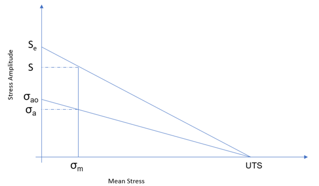
- Gerber
- Safety factor is calculated as: Where,
- Target stress amplitude corresponding to target life determined from the modified SN curve.
- Stress amplitude after mean stress correction.
Figure 6. 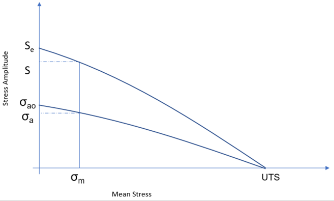
- Gerber2
- Safety factor is calculated as:
- If
:Where,
- Target stress amplitude corresponding to target life determined from the modified SN curve.
- Stress amplitude after mean stress correction.
- FKM
- Safety factor is calculated as:
Figure 7. 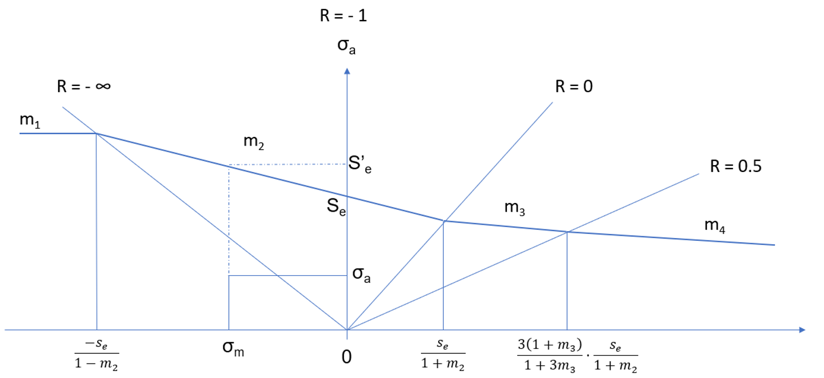
- No Mean Stress Correction
- Safety factor is calculated as:
Constant Stress Ratio Method
- Goodman
- Safety factor is calculated as:
Figure 8. 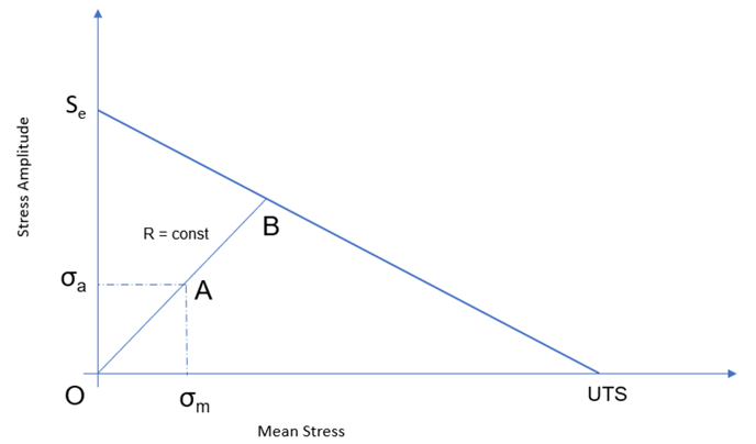
- Gerber
- Safety factor is calculated as:
- Gerber2
- Safety factor is calculated as:
- FKM
- Safety factor is calculated as:Where:
- Corrected stress amplitude in constant R mean stress correction.
- No Mean Stress Correction
- Safety factor is calculated as:
Scale Method
The scale safety factor is calculated as:
Stress for damage calculation = scale safety factor x combined stress
If the stress scaling and offset (SCALE and OFFSET on STRESS continuation on MATFAT) are defined:
Stress for damage calculation = scale safety factor x (combined stress x MATFAT scale factor + MATFAT offset)
For given events and target life, OptiStruct finds the scale safety factor that meets target life. If current life is shorter than the target life, the scale safety factor is less than 1.
If current life is longer than the target life, the scale safety factor is greater than 1. The scale safety factor is supported in EN, SN, seam weld, and spot weld time domain fatigue analysis. The scale safety factor is not supported in DangVan.
Safety Factor for Multiple SN Curves
- Multi-mean SN Curves
- To calculate safety factor, OptiStruct
creates an internal Haigh diagram for the target life using multi-mean
SN curve by finding stress amplitude-mean stress pairs at the target
life. Using the internally created Haigh diagram, OptiStruct calculates safety factor using the
method described in Chapter Haigh diagram. The number of data points of
the Haigh diagram is the number of curves. Thus the more curves
provided, the better the result given. When the Haigh diagram is not
available in mean stress ranges, the Haigh diagram is extrapolated by
OptiStruct.
Figure 9. 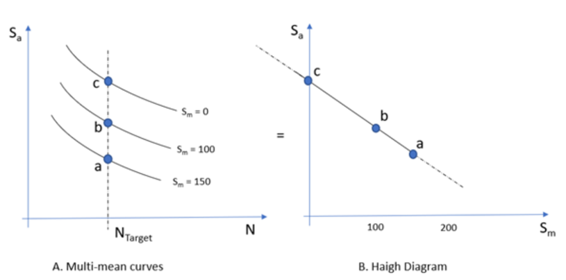
- Multi-ratio SN Curves
- To calculate safety factor, OptiStruct
create an internal Haigh diagram for the target life using multi-mean SN
curve by finding stress amplitude-mean stress pairs at the target life.
The number of data points of the Haigh diagram is the number of curves.
Thus the more curves, the better the result given. When the Haigh
diagram is not available in mean stress ranges, When Haigh diagram is
not available in mean stress ranges, the Haigh diagram is extrapolated
by OptiStruct.
Figure 10. 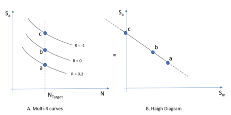
- Haigh Diagrams
- Safety factor is calculated as:
Figure 11. 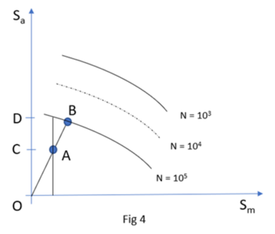
Strain-Life (E-N) Approach
Strain-life analysis is based on the fact that many critical locations such as notch roots have stress concentration, which will have obvious plastic deformation during the cyclic loading before fatigue failure. Thus, the elastic-plastic strain results are essential for performing strain-life analysis.
Neuber Correction
Neuber correction is the most popular practice to correct elastic analysis results into elastic-plastic results.
In order to derive the local stress from the nominal stress that is easier to obtain, the concentration factors are introduced such as the local stress concentration factor , and the local strain concentration factor .
Where, is the local stress, is the local strain, is the nominal stress, and is the nominal strain. If nominal stress and local stress are both elastic, the local stress concentration factor is equal to the local strain concentration factor. However, if the plastic strain is present, the relationship between and no long holds. Thereafter, focusing on this situation, Neuber introduced a theoretically elastic stress concentration factor defined as:
Substitute Equation 22 and Equation 23 into Equation 24, the theoretical stress concentration factor can be rewritten as:
Through linear static FEA, the local stress instead of nominal stress is provided, which implies the effect of the geometry in Equation 25 is removed, thus you can set as 1 and rewrite Equation 25 as:
Where, , is locally elastic stress and locally elastic strain obtained from elastic analysis, , the stress and strain at the presence of plastic strain. Both and can be calculated from Equation 26 together with the equations for the cyclic stress-strain curve and hysteresis loop.
Monotonic Stress-Strain Behavior
Relative to the current configuration, the true stress and strain relationship can be defined as:
Where, is the current cross-section area, is the current objects length, is the initial objects length, and and are the true stress and strain, respectively, Figure 12 shows the monotonic stress-strain curve in true stress-strain space. In the whole process, the stress continues increasing to a large value until the object fails at C.

The curve in Figure 12 is comprised of two typical segments, namely the elastic segment OA and plastic segment AC. The segment OA keeps the linear relationship between stress and elastic strain following Hooke Law:
Where, is elastic modulus and is elastic strain. The formula can also be rewritten as:
by expressing elastic strain in terms of stress. For most of materials, the relationship between the plastic strain and the stress can be represented by a simple power law of the form:
Where, is plastic strain, is strength coefficient, and is work hardening coefficient. Similarly, the plastic strain can be expressed in terms of stress as:
The total strain induced by loading the object up to point B or D is the sum of plastic strain and elastic strain:
Cyclic Stress-Strain Curve
- Stable state
- Cyclically hardening
- Cyclically softening
- Softening or hardening depending on strain range


- Cyclic strength coefficient
- Strain cyclic hardening exponent
Hysteresis Loop Shape
Bauschinger observed that after the initial load had caused plastic strain, load reversal caused materials to exhibit anisotropic behavior. Based on experiment evidence, Massing put forward the hypothesis that a stress-strain hysteresis loop is geometrically similar to the cyclic stress strain curve, but with twice the magnitude. This implies that when the quantity ( ) is two times of ( ), the stress-strain cycle will lie on the hysteresis loop. This can be expressed with formulas:
Expressing in terms of Δσ, in terms of Δε, and substituting it into Equation 34, the hysteresis loop formula can be calculated as:
Almost a century ago, Basquin observed the linear relationship between stress and fatigue life in log scale when the stress is limited. He put forward the following fatigue formula controlled by stress:
Where, is the stress amplitude, is the fatigue strength coefficient, and is the fatigue strength exponent. Later in the 1950s, Coffin and Manson independently proposed that plastic strain may also be related with fatigue life by a simple power law:
Where, is the plastic strain amplitude, is the fatigue ductility coefficient, and is the fatigue ductility exponent. Morrow combined the work of Basquin, Coffin and Manson to consider both elastic strain and plastic strain contribution to the fatigue life. He found out that the total strain has more direct correlation with fatigue life. By applying Hooke Law, Basquin rule can be rewritten as:
Where, is elastic strain amplitude. Total strain amplitude, which is the sum of the elastic strain and plastic stain, therefore, can be described by applying Basquin formula and Coffin-Manson formula:

Mean Stress Correction
The fatigue experiments carried out in the laboratory are always fully reversed, whereas in practice, the mean stress is inevitable, thus the fatigue law established by the fully reversed experiments must be corrected before applied to engineering problems.
Morrow is the first to consider the effect of mean stress through introducing the mean stress in fatigue strength coefficient by:
Thus, the entire fatigue life formula becomes:
Morrow's equation is consistent with the observation that mean stress effects are significant at low value of plastic strain and of little effect at high plastic strain.
Smith, Watson and Topper proposed a different method to account for the effect of mean stress by considering the maximum stress during one cycle (for convenience, this method is called SWT in the following). In this case, the damage parameter is modified as the product of the maximum stress and strain amplitude in one cycle.
The SWT method will predict that no damage will occur when the maximum stress is zero or negative, which is not consistent with the reality.
When comparing the two methods, the SWT method predicted conservative life for loads predominantly tensile, whereas, the Morrow approach provides more realistic results when the load is predominantly compressive.
Damage Accumulation Model
In the E-N approach, use the same damage accumulation model as the S-N approach, which is Palmgren-Miner's linear damage summation rule.