Composite Analysis
In this tutorial, you will complete a model build process for a typical composite model.
This tutorial covers all steps to get from meshed geometry to a fully defined composite model.
Open the Model and Composite Browser
- Start HyperMesh.
- From the menu bar, click .
-
Browse to your working directory, select composite_hat.hm,
and click Open.
The model opens in the modeling window.
-
From the Model ribbon, select the
Composites tool.
Figure 2. 
The Composite Browser opens.
Define Stacking Direction
Define the stacking direction of plies in the laminate.
-
Right-click in the white space of the Composite Browser and
select from the context menu.
The Material Reference Orientation dialog opens.
- In the Normals tab, select elements by clicking Elements and selecting all elements in the hat.
-
In the microdialog, click
 .
.
-
In the Material Reference Orientation dialog, click
Apply.
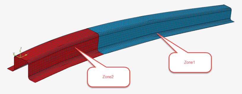
Current element normals for 2D elements are displayed. Notice the direction of the current element normals. In this example, the elements in the model represent the OML of the part, and accordingly, the plies stack inward. To model this, the element normals must be flipped to properly represent the stacking direction of the laminate from the tooling surface.
-
For Operation section, choose Reverse then click
Apply to flip the direction of the element
normals.
Figure 3. 
Figure 4. 
- Click Clear to remove the element normal vector plot.
Define Material Orientation
Define the x material reference orientation for the part.
- In the Reference Orientation tab of the Material Reference Orientation dialog, select the elements on which material orientation will be set by clicking Elements and selecting all elements in the tapered_beam component.
-
In the microdialog, click .
- For X direction method, select System.
-
In the microdialog, select the local system in the
material_reference_system collector, then click .
-
In the microdialog, click .
-
Click Apply and close the Material Reference
Orientation dialog.
Note: The user profile and orientation method will determine the final solver cards created or manipulated. In this case specifically, in OptiStruct the MCID field of the element cards will be populated by the system id. Internally, OptiStruct will project the system x-axis onto the elements to define the material x direction.
Figure 5. 
Figure 6. 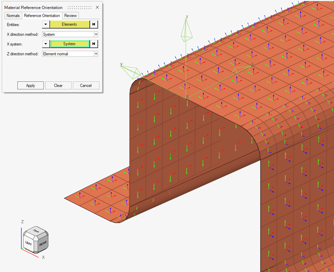
Material Creation
Create new materials and review existing materials.
-
To create a material, right-click in the white space of the Composite Browser, and select from the context menu.
A material entity with the appropriate card for the selected user profile is created. This material can be left in the database or deleted, this tutorial will use existing materials.
-
In the Composite Browser, select the
carbon_epoxy material and review the material
properties in the Entity Editor.
Note:
- These properties are typical of a uni-direction carbon-epoxy product in mmNS consistent units.
- In the OptiStruct user profile, MAT9OR cards are used to define orthotropic shell material properties.
- Repeat steps 1 and 2 to review the glass_epoxy material properties.
-
Note if exact material properties are not available; Multiscale Designer can be used to generate typical homogenized material
properties from a selection of fiber, matrix, and volume fraction.
Figure 7. 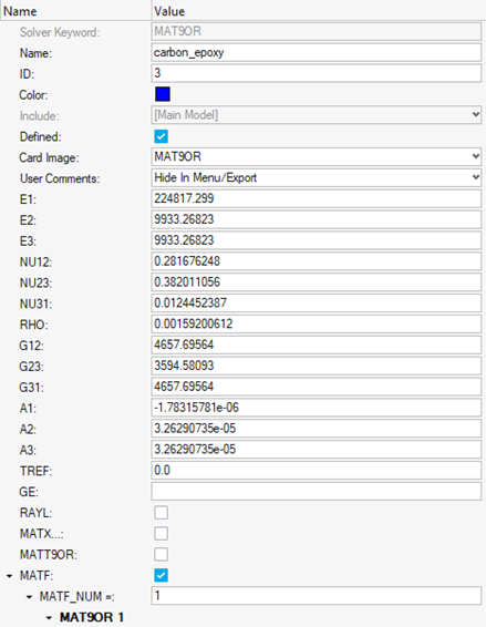
Ply Creation
Create the plies that make up the composite laminate.
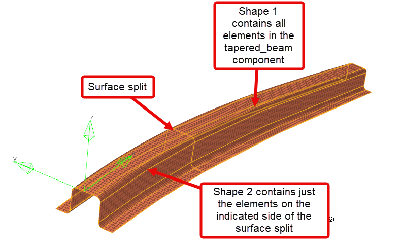
-
Define Shape1 and Shape2.
Shapes can be assigned to one or multiple plies by selecting plies in the Composite Browser and populating the Shape field in the Entity Editor.The new shapes appear in the Composite Browser.
-
Create uni-directional plies.
Note: Multiple plies can be Ctrl or Shift selected to edit multiple values at once.
Table 1. Uni-Directional Ply Details Ply Name Ply ID Thickness Orientation Material Shape uni_1 1 0.2 0 carbon_epoxy Shape1 uni_2 2 0.2 90 carbon_epoxy Shape1 uni_3 3 0.2 90 carbon_epoxy Shape2 uni_4 4 0.2 0 carbon_epoxy Shape2 -
Repeat steps 2.a - 2.g to create woven plies using the values in Table 2.
In addition to values set in step 2, the Ply type should be set to Unidirectional Weave. This method uses a material model with properties at the scale of the warp/weft direction – the material properties are the unidirectional equivalent after dehomogenizing homogenized properties where E1=E2. The unidirectional weave ply type internally uses four unidirectional plies with 0.25 thickness, where the stacking sequence is [θ/θ+90/θ+90/θ].Note: If you do not know these properties but wish to use this ply type, you can use the homogenized weave ply type instead. If these plies are then changed to unidirectional weave or are draped, the material will be dehomogenized automatically.
Table 2. Woven Ply Details Ply Name Ply ID Thickness Orientation Material Shape woven_1 5 0.18 45 glass_epoxy Shape1 woven_2 6 0.18 45 glass_epoxy Shape1 -
Select all the created plies in the Composite Browser,
select one of the color icons, and click
 to apply auto
color.
to apply auto
color.
Figure 9. 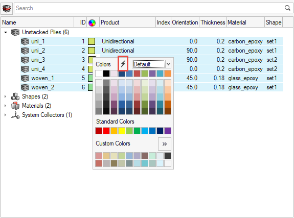
Laminate Creation
Create the laminate and stack the plies.
- In the Composite Browser, right-click in white space and select from the context menu.
-
In the Entity Editor, confirm
STACK is selected for Card Image.
This will set the card that defines the laminate in OptiStruct. In other solvers, this will be None.
-
In the Entity Editor, confirm
Total is selected for Laminate Option.
This specifies that the ABD matrix calculated from the laminate will be exact. Other common options include:
- Smear: removes the effect of stacking sequence from the ABD matrix.
- Symmetric: allows only half the plies to be modeled. The other half will be managed automatically.
- Shift select all the plies created in Ply Creation and drag-and-drop them into the laminate.
-
Reorganize the stacking sequence of the laminate so it matches Figure 10 by
dragging-and-dropping plies within the laminate.
Figure 10. 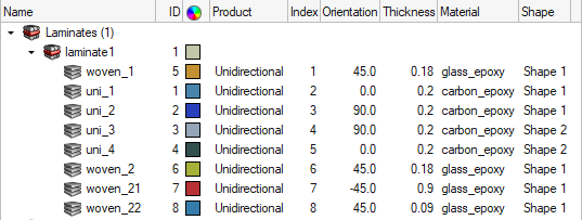 Note: Plies can also be automatically created from a spreadsheet import. Created plies can be exported to a spreadsheet. To access this functionality, right-click on a laminate and select Import or Export CSV.
Ply-Based Property Creation
Create the ply-based property, which specifies solver property card-specific attributes.
- In the Composite Browser, right-click in the white space and select from the context menu.
-
In the Entity Editor, verify that
PCOMPP is selected for Card Image.
For other solvers, the card image will be the typical zone-based composite property.
-
In the Entity Editor, verify Z0 to set to
0.0.
In OptiStruct, this defines the offset such that plies begin stacking from the location in space of the elements.
- Assign PCOMPP to the elements of the tapered_ beam component. Right-click on the property and select Assign from the context menu.
-
Select the tapered_beam component, then click on the
guide bar to assign the property and exit the
tool.
Figure 11. 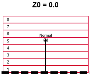
Note: No other information about the composite property layers needs to be set, regardless of solver. All layer information is defined on the ply and laminate entities.
Material Reference Orientation Visualization
Plot vectors which visualize the x,y,z reference orientation.
-
From the Composite Browser, right-click a laminate and
select from the context menu.
The x,y,z reference orientations are plot on each element contained in the ply or laminate.
Figure 12. 
-
Repeat step 1 to deactivate the Material Reference option.
Note: For additional control over which elements vectors are plotted on and which vectors are drawn, the Material Reference Orientation dialog can be used.
- From the Composite Browser, right-click the white space and select from the context menu.
- Select elements, axis visibility, axis color, and vector scaling as desired and click Apply to plot the vectors.
Ply Direction Visualization
Plot vectors which visualize the ply 1 direction/fiber direction.
- From the Composite Browser, right-click a ply and select from the context menu.
-
Select other plies in the Composite Browser.
Note: For the unidirectional weave ply type, both the warp and weft fiber directions will be plotted.The ply 1 direction (fiber direction) is plotted at each element.
- Repeat step 1 to deactivate the Ply 1 Direction option.
-
For additional control over which vectors are plotted, right-click the white
space of the Composite Browser and select from the context menu.
The Orientation Review dialog opens at the Ply directions tab. Vector display of fiber orientation, draped fiber orientation, x, y, and z orientations and other coloring and scaling options can be set here.
Figure 13. 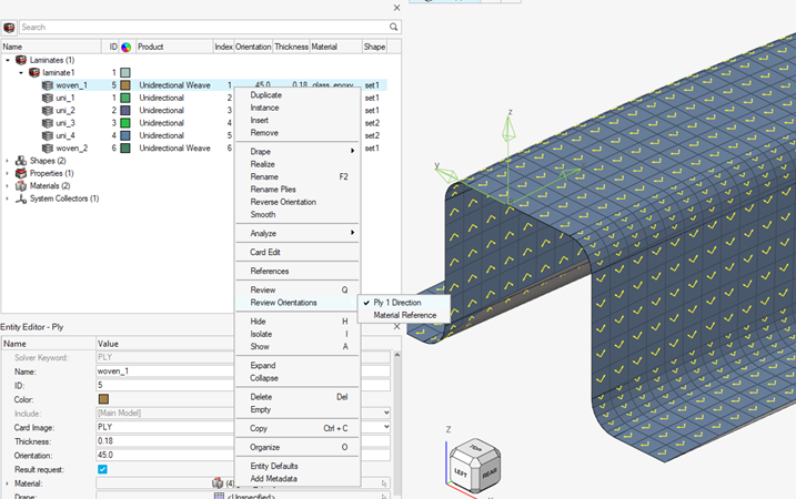
Ply Shape Visualization
Plot the shape boundary of each ply.
- From the Composite Browser, select one or more
plies
This will draw the boundary of the ply shape for each selected ply.
- From the Composite Browser, right-click one ply and
select Review from the context menu.
This will highlight all elements of the shape of the selected ply.

Thickness and Layers Visualization
Visualize the thickness and ply layers of the laminate.
- Open the Element and Handle Visualization dialog at the bottom of the graphics area.
- Activate 3D and Ply Layers.
-
From the menu bar, select and enter 5 in the ply visualization
thickness factor input.
Figure 15.  This will temporarily increase the displayed thickness of each ply layer for the purposes of visualization.
Result Requests
Request typical composite results from OptiStruct.
-
In the Model Browser, right-click in white space and select
Create from the context menu.
The Create Entity dialog opens.
-
Select Cards from the Entities selection on the left
tree, select GLOBAL_OUTPUT_REQUEST from the right tree,
and click Create.
Note: In OptiStruct, results can also be requested for each subcase.
-
Request ply level strains by selecting CSTRAIN and set
the following options:
- EXTRA = MECH – this will request mechanical strains, which cause stress
- NDIV = 3 – this will output results at the top, middle, and bottom of each ply
- OPTION = YES – this will request the output
-
Request ply level stresses by selecting CSTRESS and set
the following options:
- NDIV = 3 – this will output results at the top and bottom of each ply
- OPTION = YES – this will request the output
-
Request the first ply failure/onset by checking CFAILURE. Set the following
options:
- NDIV = 3 – this will output results at the top and bottom of each ply
- OPTION = YES – this will request the output
This will print first ply failure results using the allowables defined on the MAT9OR material card and failure theory specified on MATF CRITERIA field.Figure 16. 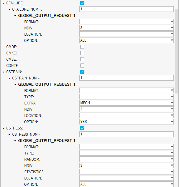
Draping
Perform a draping simulation to account for local orientation changes in each ply due to compound curvature.
-
In the Composite Browser, right-click the
laminate1 folder and select from the context menu.
This opens the Kinematic Draping tool and performs a draping simulation on all plies.Note: Plies can also be draped individually or in small numbers by Shift-selecting them directly.
- Double-click the Node collector to select the Seed point.
-
Select Node 4173.
This is the location where the ply first touches the tool during manufacturing.
- Confirm the Method is set to Quadrants.
- Click Apply to drape the plies.
- Repeat the Ply Direction Visualization step to visualize the draping results.
-
Before clicking Apply, check
the Drape fiber orientation.
Note: Draping simulation generates a DRAPE table for each ply draped. The table contains thickness and orientation corrections for each element.
Figure 17. 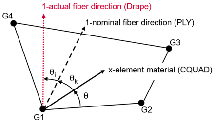
Laminate Realization and Solver Property Creation
Generate zone-based solver properties from the ply-based model.
This step is typically performed at the end of a model build for solvers other than OptiStruct because those solvers do not directly support ply-based property cards. OptiStruct directly supports ply-based laminate and ply cards and therefore this step can be omitted in the OptiStruct profile unless PCOMPGs are required.
- In the Composite Browser, right-click the Laminates folder and select Realize from the context menu.
-
Clear the Include drape option and select
Realize.
Notice the new properties generated and assigned to the model.
Figure 18. 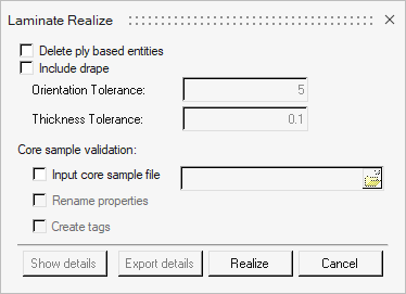
Figure 19.