Apply Forces

Create concentrated forces by applying a load, representing forces, to a node or set.

Forces are load config 1 and are displayed as a vector with the letter F at the tail end.

Note: In the Radioss, Abaqus, and LS-DYNA profiles, load entities are created immediately upon entering the tool. Use the Entity Editor to modify any properties. In all other solver profiles, load entities aren't created until you make your selections then click Create.

From the Analyze ribbon, Loads tool group, click the Forces tool.

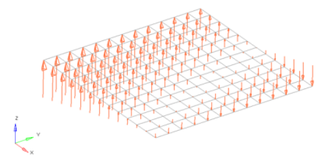
Figure 1.
Select the keyword to create from the Load Type menu.
The available types depend on the current solver interface.
Choose the entities to which the force will be applied.
Choose whether to create the forces in the global system or a local system.
Specify the magnitude and direction of the force.

Constant Components

Specify the direction and magnitude of the load by entering the X, Y, and Z values of the components.

Constant Vector

Specify the magnitude, then use the plane and vector tool to specify the vector along which the load should act.

Curve Components

Specify the X, Y, and Z components to define the direction and magnitude, for example, (2,2,2) will be twice the magnitude of (1,1,1). Next, select an existing curve. Last, specify a factor for the curve’s xscale to use the same curve for many different cases, but vary the scale of its intensity or time to match the needs of your current load.

Curve Vector

When working with loads that are time dependent, use this method to first specify a magnitude (yscale) for the curve. Next, select an existing curve, then use the plane and vector tool to specify a direction, if necessary. Last, specify a factor for the curve's xscale to use the same curve for many different cases, but vary the scale of its intensity or time to match the needs of your current moment.

Equation

Specify the loading equation. Use the plane and vector tool to specify a direction, then select the coordinate system to which the vector corresponds.

Field Loads

Interpolate and extrapolate loads from existing loads. You can then select the desired elements to which you wish to add loads, and any existing loads on which you wish to base additional forces.

When you create, HyperMesh uses a Green's function with the given boundary loads in order to create the loads on all of the selected nodes. For smoothness, the gradient at the boundary points is enforced to be zero; this ensures that the extrapolated loads remain lower than the input loads. For this reason it is recommended to use representative boundary values as input to be able to capture the peaks reasonably.
Note: This version differs from linear interpolation both in the way that the load magnitudes are determined, and also in the fact that it can be applied to nodes outside the boundaries of the chosen existing loads.

Linear Interpolation

Interpolate loads from a saved file or existing loads.
Note: Only available for shell elements.

Each row of the input file contains the x,y,z coordinates of the load followed by its three components. The data can be separated by a space or tab.

You can then select the desired nodes to which you wish to add loads, and pick 3 or more existing loads that enclose those nodes. When you interpolate, a linear function is used to create additional loads on the selected nodes, with magnitudes based on the magnitudes of the loads that you had selected.

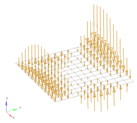
Figure 2.

In the search radius field, specify the search distance to find the loads which are within that distance from a centroid or node on which a load is being interpolated. The nearest 3 loads located within that distance are used to create the load at the centroid or node by linear interpolation. Linear interpolation uses a triangulation method, so if it finds fewer than 3 loads within that distance no interpolation takes place. While reading the initial loads from a file, if linear interpolation is not possible because the search radius is too small, the original loads are simply applied to the nearest centroid or node.

Select fill gap to create a load at every selected element centroid or node irrespective of the size of the search radius.

Nodal distribution

Specify the magnitude, then use the plane and vector tool to specify the vector along which the load should act.

If you do not specify a vector using the plane and vector tool, the force will be normal to the selected nodes' adjacent surfaces by default.

Loads from files formatted as CSV (Comma Separated Values) or SSV (Space-Separated Values) text files can be interpolated.

Field Loads will not overwrite any existing loads, so you can create an area of loads via linear interpolation and then use field loads to expand the load area without changing the loads already inside of the area.
If working in a controller, click Create.

Equations allow you to create force, moment, pressure, temperature or flux loads on your model where the magnitude of the load is a function of the coordinates of the entity to which it is applied. An example of such a load might be an applied temperature whose intensity dissipates as a function of distance from the application point, or a pressure on a container walls due to the level of a fluid inside.

Functions must be of the form magnitude= f(x,y,z). The only variables allowed are x, y and z, (lower case) which are substituted with the coordinate values of the entity to which the load is applied. In the case of grid point loads (force, moment or temperature) the grid point coordinates are used. For elemental loads (pressure or flux) the element centroid coordinates are used. In the event that a cylindrical or spherical coordinate system is used, x, y and z are still used to reference the corresponding direction. Standard mathematical operators and functions can be used; however, any functions requiring external data will not be valid.

Note: If your equation contains a syntax error, no warning message will be displayed, but any loads created will have a zero magnitude.