Apply Flux Loads

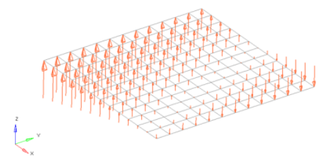
Create concentrated fluxes by applying a load, representing fluxes, to element nodes.

1. From the Analyze ribbon, click the Flux tool.

   
   
   Figure 1.

2. Select the keyword to create from the Load Type menu.
   The available types depend on the current solver interface.
3. Select entities to which temperatures will be applied.
   In any case, the forces are applied to nodes; this selection simply determines how those nodes are selected. For example, elements select the nodes at the corner of each element picked.
4. Specify the magnitude and direction of the temperature.

   Constant Value

   The value of the load magnitude.

   Curve

   Select a curve, then specify the value (y scale) to apply to the curve. Optionally, you can enter an xscale if your solver supports it.

   Equation

   Specify the loading equation. Use the plane and vector tool to specify a direction, then select the coordinate system to which the vector corresponds.

   Field Loads

   Interpolate and extrapolate loads from existing loads. You can then select the desired elements to which you wish to add loads, and any existing loads on which you wish to base additional forces.

   When you create, HyperMesh uses a Green's function with the given boundary loads in order to create the loads on all of the selected nodes. For smoothness, the gradient at the boundary points is enforced to be zero; this ensures that the extrapolated loads remain lower than the input loads. For this reason it is recommended to use representative boundary values as input to be able to capture the peaks reasonably.

   Note: This version differs from linear interpolation both in the way that the load magnitudes are determined, and also in the fact that it can be applied to nodes outside the boundaries of the chosen existing loads.

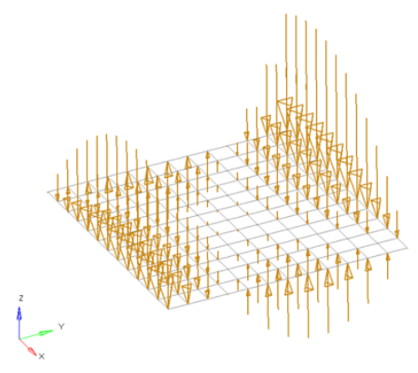
   Linear Interpolation

   Interpolate loads from a saved file or existing loads.

   Note: Only available for shell elements.

   Each row of the input file contains the x,y,z coordinates of the load followed by its three components. The data can be separated by a space or tab.

   You can then select the desired nodes to which you wish to add loads, and pick 3 or more existing loads that enclose those nodes. When you interpolate, a linear function is used to create additional loads on the selected nodes, with magnitudes based on the magnitudes of the loads that you had selected.

   
   
   Figure 2.

   In the search radius field, specify the search distance to find the loads which are within that distance from a centroid or node on which a load is being interpolated. The nearest 3 loads located within that distance are used to create the load at the centroid or node by linear interpolation. Linear interpolation uses a triangulation method, so if it finds fewer than 3 loads within that distance no interpolation takes place. While reading the initial loads from a file, if linear interpolation is not possible because the search radius is too small, the original loads are simply applied to the nearest centroid or node.

   Select fill gap to create a load at every selected element centroid or node irrespective of the size of the search radius.

   Loads from files formatted as CSV (Comma Separated Values) or SSV (Space-Separated Values) text files can be interpolated.

   Field Loads will not overwrite any existing loads, so you can create an area of loads via linear interpolation and then use field loads to expand the load area without changing the loads already inside of the area.

5. If working in a controller, click Create.

Equations allow you to create force, moment, pressure, temperature or flux loads on your model where the magnitude of the load is a function of the coordinates of the entity to which it is applied. An example of such a load might be an applied temperature whose intensity dissipates as a function of distance from the application point, or a pressure on a container walls due to the level of a fluid inside.

Functions must be of the form magnitude= f(x,y,z). The only variables allowed are x, y and z, (lower case) which are substituted with the coordinate values of the entity to which the load is applied. In the case of grid point loads (force, moment or temperature) the grid point coordinates are used. For elemental loads (pressure or flux) the element centroid coordinates are used. In the event that a cylindrical or spherical coordinate system is used, x, y and z are still used to reference the corresponding direction. Standard mathematical operators and functions can be used; however, any functions requiring external data will not be valid.

Note: If your equation contains a syntax error, no warning message will be displayed, but any loads created will have a zero magnitude.

Figure 3. Flat Plate with a Linear Function for an Applied Force Magnitude = 20 – (5*x+2*y). The flat plate is 20 x 20 units, lying in the X-Y plane with the origin at the center.

Figure 4. Flat Plate with a Polynomial Function with Magnitude = x^2-2y^2+x*y+x+y. The flat plate is 20 x 20 units, lying in the X-Y plane with the origin at the center.

Figure 5. Curved Surface with a Polynomial Function for an Applied Pressure Magnitude = -((x^2+2*y^2+z)/1000). The pressure function is defined in terms of the cylindrical coordinate system displayed at the top edge of the elements.