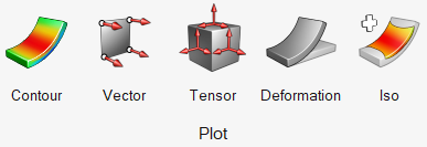
Results can be visualized in the form of contour, vector, tensor, deformation, and iso
plots using the corresponding tools available in Plot Ribbon.Figure 1.
Each of these tools launches a guide bar that will
take the you through the steps required for plotting a particular type of plot.
View Contour Plots
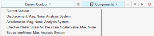
From the Plot Ribbon, click the Contour tool.
Figure 2.
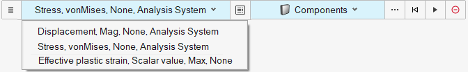
The Contour guide bar opens.
Select a definition to be contoured from the list.
Figure 3. To understand the difference between Current Contour item and the other
definitions in the list (see the Current Plot versus Definitions
section).
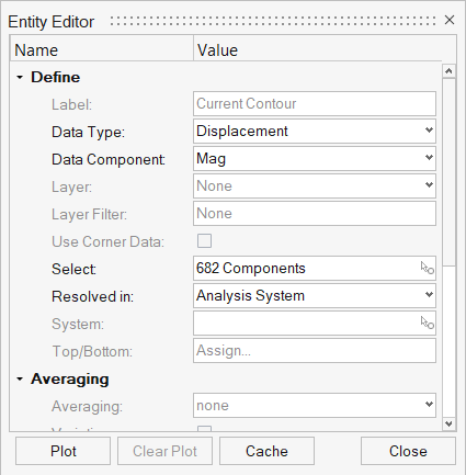
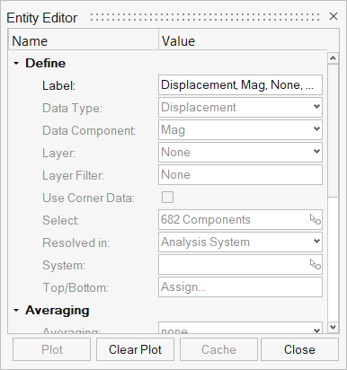
Optional: Click on the View/Edit button to see the details of a
selected definition.
In the case of current contour, the definition can be edited.
In the case of
other definitions, if they are cached already, then only the label can be
changed, and rest of the fields are non-editable.
The dialog also has
buttons for Plot/Clear
Plot/Cache located at the bottom.Figure 4.
Optional: Click on the entity selector to select the entities on which the plot will be
displayed.
The entities can be selected by any of the available selection methods:
graphical picking, by window, by advanced selection. Entities can be selected
across overlaid models by graphical picking, by window, and by quick selection
(right-click context menu Select > Displayed/Reverse/All).
Note: This entity selector acts as a
display filter allowing you to show the contour plot on only a subset of the
entities for which the definition has been loaded (which is typically all
the components in the model). The rest of the entities will be shown in
grey, however the data is still available for query.
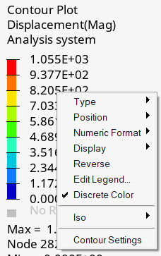
Click the Plot button to view the contour plot of the
selected definition.
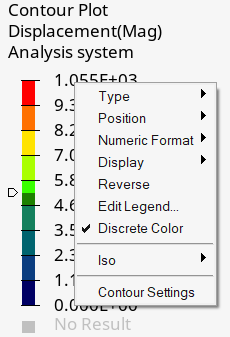
A legend is displayed on the screen along with the plot. Right-click on the
legend to access a context menu with options to update the legend and contour
display settings.
Figure 5.
Click the Clear Plot button to remove the plot from
display.
If the tool is exited without clicking the Clear Plot button, then the plot
remains displayed.
Click the Esc key or click on the
Contour icon again to exit the tool.
View Vector Plots
From the Plot Ribbon, click the Vector tool.
Figure 6.
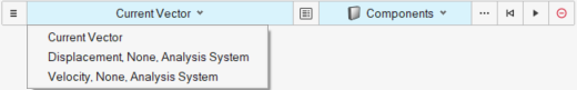
The Vector guide bar opens.
Select a definition from the list.
Figure 7. To understand the difference between Current Vector item and the other
definitions in the list (see the Current Plot versus Definitions
section).
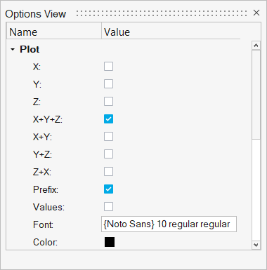
You can also set some Vector Plot Display options upfront by clicking on the
Options button on the left of the guide bar.Figure 8.
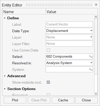
Optional: Click on the View/Edit button to see the details of a
selected definition.
In the case of current vector, the definition can be edited.
In the case of
other definitions, if they are cached already, then only the label can be
changed, and rest of the fields are non-editable.
The dialog also has
buttons for Plot/Clear
Plot/Cache located at the
bottom.
Figure 9.
Optional: Click on the entity selector to select the entities on which the plot will be
displayed.
The entities can be selected by any of the available selection methods:
graphical picking, by window, by quick or advanced selection. Entities can be
selected across overlaid models by graphical picking, by window, and by quick
selection (right-click context menu Select > Displayed/Reverse/All).
Note: This entity selector acts as a
display filter allowing you to show the vector plot on only a subset of the
entities for which the definition has been loaded (which is typically all
the components in the model). Plot will not be displayed on the rest of the
entities; however, the data is still available for query.
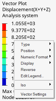
Click the Plot button to view the vector plot of the
selected definition.
A legend is displayed on the screen along with the plot. Right-click on the
legend to access a context menu with options to update the legend and vector
display settings.
Figure 10.
Click the Clear Plot button to remove the plot from
display.
If the tool is exited without clicking the Clear Plot button, then the plot
remains displayed.
Click the Esc key or click on the
Vector icon again to exit the tool.
View Tensor Plots
From the Plot Ribbon, click the Tensor tool.
Figure 11.
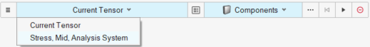
The Tensor guide bar opens.
Select a definition from the list.
Figure 12. To understand the difference between Current Tensor item and the other
definitions in the list (see the Current Plot versus Definitions
section).
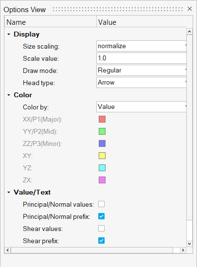
You can also set some Tensor Plot Display options upfront by clicking on the
Options button on the left of the guide bar.Figure 13.
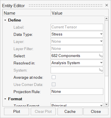
Optional: Click on the View/Edit button to see the details of a
selected definition.
In the case of the current tensor, the definition can be edited.
In the case
of other definitions, if they are cached already, then only the label can be
changed and rest of the fields are non-editable.
The dialog also has
buttons for Plot/Clear
Plot/Cache located at the
bottom.
Figure 14.
Optional: Click on the entity selector to select the entities on which the plot will be
displayed.
The entities can be selected by any of the available selection methods:
graphical picking, by window, by quick or advanced selection. Entities can be
selected across overlaid models by graphical picking, by window, and by quick
selection (right-click context menu Select > Displayed/Reverse/All).
Note: This entity selector acts as a
display filter allowing you to show the tensor plot on only a subset of the
entities for which the definition has been loaded (which is typically all
the components in the model). Plot will not be displayed on the rest of the
entities; however, the data is still available for query.
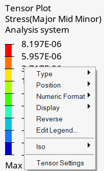
Click the Plot button to view the tensor plot of the
selected definition.
A legend is displayed on the screen along with the plot. Right-click on the
legend to access a context menu with options to update the legend and tensor
display settings.
Figure 15.
Click the Clear Plot button to remove the plot from
display.
If the tool is exited without clicking the Clear Plot button, then the plot
remains displayed.
Click the Esc key or click on the
Tensor icon again to exit the tool.
View Iso Plots
From the Plot Ribbon, click the Iso tool.
Figure 16.
The Iso guide bar opens.
Select a definition to apply an iso plot to from the list.
Note: In the case of an Iso plot, current Iso is not available, and a
definition is required to create an iso plot. Therefore, it is important to
make sure that definitions are loaded upfront or that the current contour is
cached to create an iso plot.
To understand the difference between
the Current Plot item and the other definitions in the list (see the
Current Plot versus Definitions section).
Figure 17.
You can also set some Iso Plot Display options upfront by clicking on the
Options button on the left of the guide bar.
Optional: Click on the View/Edit button to see the details of a
selected definition.
If the definitions are cached, then only the label can be changed and rest of
the fields are non-editable.
The dialog also has buttons for Plot/Clear
Plot/Cache located at the bottom.
Figure 18.
Optional: Click on the entity selector to select the entities on which the plot will be
displayed.
The entities can be selected by any of the available selection methods:
graphical picking, by window, by quick or advanced selection. Entities can be
selected across overlaid models by graphical picking, by window, and by quick
selection (right-click context menu Select > Displayed/Reverse/All).
Note: This entity selector acts as a
display filter allowing you to show the iso plot on only a subset of the
entities for which the definition has been loaded (which is typically all
the components in the model). Iso plot will not be displayed on the rest of
the entities.
Click the Plot button to view the iso plot of the
selected definition.
If a matching contour plot is present, then a slider is displayed in the legend
which can be used to control the iso plot display. Additional iso options are
also available using the Legend right-click context menu.
Figure 19.
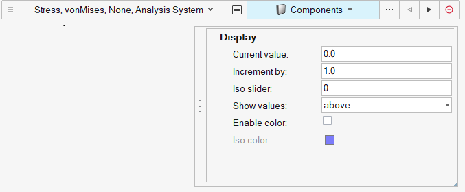
If the contour plot is not present or does not match the iso plot, then a
micro dialog to control the iso plot display will be displayed.Figure 20.
Click the Clear Plot button to remove the plot from
display.
If the tool is exited without clicking the Clear Plot button, then the plot
remains displayed.
Click the Esc key or click on the
Iso icon again to exit the tool.
Tip: A results plotting workflow is also possible using the HyperViewResults Browser, although some of the plotting options are
available only through the Plot guide bars.
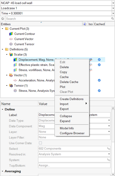
The Results folder in the browser
lists all the definitions available and through the icons or right-click context
menu, you can Plot or Clear Plot of any definition. Additional context menu
options to Cache/Delete Cache/Delete a definition, and so on are available. Figure 21.
View Deformation Plots
From the Plot Ribbon, click the Deformation tool.
Figure 22.
The Deformation guide bar opens.
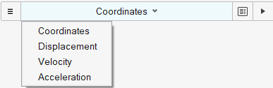
Select a result type to be used as the deformation type (animation
source).
Note:
In the case of some crash solvers such as LS-DYNA or Radioss,
animation data is available in the form of coordinates and it will
be used as the default data type. It is recommended to use this for
better performance.
Deformation data is not permanently cached, therefore when the type
is changed and replotted, old data is discarded and new data is read
from the file.
Figure 23.
You can also set some Undeformed shape options upfront by clicking on the
Options button on the left of the guide bar.
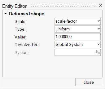
Click on the View/Edit button to view and set the
deformation shape parameters.
Figure 24.
Click the Plot button to view the deformation based on
the current setting.
Click the Esc key or click on the
Deformation icon again to exit the tool.
Current Plot versus Definitions
Two options are available when it comes to loading and viewing results as contour, vector,
or tensor plots.
Current Plot: This is an 'on-demand' approach to plotting. The plot guide bar will
show an item named “Current Contour” (or Vector or Tensor) in the definitions list. You
can simply use this item to plot any result type. Data will be loaded from the file at
the time of plotting. If you want to plot a different result, use the View/Edit button
in the guide bar to change the “Current Contour” (or Vector or Tensor) definition and
plot again. Previously plotted results will be cleared from memory and the new result
will be now be plotted.
Note:
With Current Plot, data remains in memory only if the plot is displayed. If you
clear the plot or edit the definition to view a different result, data is again
read from the file.
If you want to save the current plot for future access, you can click the Cache
button available in the View/Edit dialog. A cached entry is created under the
definitions list with a default label specifying the
datatype/component/layer/resolved in system.
The current plot workflow follows the same 'on-demand' approach as the
contour/vector/tensor panels in standard HyperView
(non-MultiCore mode).
There is a relationship between the current folder items and definition folder
items. When you plot any definition from the definitions folder, depending on its
type, the corresponding current item is updated and shown as plotted (the plot
icon is highlighted in browser). Similarly, when a current item is plotted, any
cached entry created from it is also shown as plotted.
Definitions: This is the new 'upfront' approach to plotting. Define upfront what you
would like to view as a contour, vector, iso or tensor plot using the Definitions tab in
the Load Data dialog. The definitions are loaded and remain cached in memory whether the
plot is displayed or not. The Plot Guide bars will list all the cached definitions and
you can simply choose any one of them to plot and it will be displayed instantly as no
data is read from the file.
Definitions can be created using one of the following methods:
Load Data Dialog Definitions Tab
"+" satellite icon available on hovering over the main icon in the Plot Ribbon
Right-click Context Menu option in the Results Browser
Import an XML File
Create Definitions Dialog
This dialog allows you to create multiple definitions across data types at one
time.
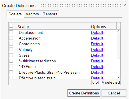
Figure 25.
Results in the file are grouped into Scalars, Vectors, and Tensors tabs. The
options column allows you further select the necessary sub-types such as data
components, data layers, resolved in systems, and so on. A default set of options is
selected for each result (for example, displacement will automatically create a
definition of displacement magnitude in the analysis system and stress defaults to
vonMises).
You can select multiple definitions to create and edit them by changing the
"default" settings in the Create Definitions dialog.
Note: Created definitions can be
deleted by selecting them in them in the browser and right-clicking and selecting
Delete from the context menu.
One of the advantages of using this dialog is that it allows you to create multiple
definitions of a specific data type very quickly. For example, in the figure below,
three components, two layers and two resolved in systems have been selected under
data type stress. This will create twelve definitions of type stress in a single
step.
Attention: Creating too many definitions may cause some application slow
down.
Once definitions are created, they can further be edited by selecting a result
definition in the browser and editing its attributes in the Entity Editor.
Restriction: Only the
definitions that have not been loaded can be edited.
Definition labels are auto generated based on the following scheme:
<datatype_name>, <datatype_component>, <datatype_layer>, <resolved in
system>. If any of these are not present for that data type, 'None' is used in the
label. If the definition attributes are edited, the label is not auto updated. You
are free to rename the label.
Note: The Create definitions dialog prevents duplicate
definitions from getting created by checking if definitions with same attributes
are already present.Figure 26.
Import XML Files Containing Definitions
Definitions that have been created can be exported and reused on a different model
easily. Simply select and right-click on the definitions that you want to reuse and
click Export, save it to an XML file, and import it on a new
model. You can choose to either append or replace the existing definitions or replace
them.
The preference statement, *DefaultResultDefinitionFile,
defined in the preferences_post.mvw file, allows you to point
to an XML file containing definitions, thus saving the time required to manually
create the definitions each time. Every time a model is loaded into the session, the
definitions contained in the file are automatically created and shown in the Results
folder.
Tip:HyperView only checks if the
data type and component necessary to create the definition are available in the
file. You are therefore expected to set this option only when you load files
containing all the relevant data required to create the definitions.
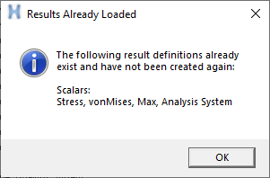
Updating Result Definitions
In the HyperView - MultiCore profile, result definitions are
cached only for the animation steps that have been loaded in the Loadcase tab. If additional
steps/frames are loaded at a later stage, the cached (but not plotted) definitions are not
automatically updated. You will see the green check mark on the cached definitions turning
into a partially loaded progress bar, indicating that the data is not available for the
additional steps. Also, if you plot a cached definition and animate, you will see an N/A
plot on the additional frames. To get the data for the additional steps, simply cache the
definition again.
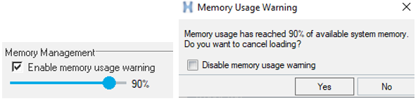
Memory Monitoring
Memory monitoring is a useful feature available only in the HyperView - MultiCore profile. It is enabled by default and can be
turned off by going to Preferences > Options dialog, clicking on Performance tab and clearing the
check box.
If it is enabled, the tool monitors total system memory (RAM) usage when any HyperView application is loading data. Once usage reaches the set
threshold, a warning dialog is shown asking if you want to cancel loading. Figure 27.
Note: If you select No without checking the Disable memory usage warning box, then the
tool continues to monitor memory usage and will pop up the dialog at approximately 5%
increments.
Once memory usage reaches 100%, the operating system starts swapping and this will cause
the cause the system to slow down. Therefore, it is recommended that the monitoring is kept
enabled with an optimum threshold value.
Once loading is canceled, the monitoring threshold gets set to the percentage at which it
was canceled so that the next time any data is loaded, the tool uses this new value as the
threshold.