Since version 2026, Flux 3D and Flux PEEC are no longer available.
Please use SimLab to create a new 3D project or to import an existing Flux 3D project.
Please use SimLab to create a new PEEC project (not possible to import an existing Flux PEEC project).
/!\ Documentation updates are in progress – some mentions of 3D may still appear.
Local post processing : graphical representation (isovalues, isolines, arrows)
Introduction
To facilitate the results post processing, the representation of the usual quantities (the most frequently used ones) is prerecorded * at the level of the data base and directly accessible from the data tree.
Thus, it is possible to quickly access the representation of the magnetic flux density on the entire computation domain, or of the electrical potential on the device, …
These elements are presented in detail in the following sections.
- prerecorded does not mean that the results of the calculation are stored
- prerecorded means that the information concerning the support for the representation and the local quantity are stored
Prerecorded graphic representation *: definition
A prerecorded graphic representation * contains :
-
a predefined space group:
the finite element computation domain (domain) / the device (no_vacuum)
- a usual local quantity, which depends on the physical application : magnetic flux density B, electrical potential V, temperature T, …
The usual local quantities are listed in the tables below.
| Application |
1_isoval_domain 2_isoval_no_vacuum |
1_isolin_domain 2_isolin_no_vacuum |
1_arrow_domain 2_arrow_no_vacuum |
|---|---|---|---|
| Isovalues | Isolines | Arrows | |
| Magneto Static |
|
An → 2D plane 2ð.rAn → 2D axi
|
|
| Transient Magnetic |
|
An → 2D plane 2ð.rAn → 2D axi Re( |
|
| Steady State AC Magnetic | Re( |
Re(An) → 2D plane Re(2ð.rAn) → 2D axi Re( |
|
| Electro Static |
|
Ve |
|
| Electric Conduction |
|
Ve |
|
| Steady State AC Electric | Re( |
Re(Ve) |
|
| Steady State Thermal | Temp(TKelvin) | Temp(TKelvin) |
|
| Transient Thermal | Temp(TKelvin) | Temp(TKelvin) |
|
| Steady State AC Magnetic coupled with Transient Thermal (3D) | Re( |
Re( |
|
- prerecorded does not mean that the results of the calculation are stored
- prerecorded means that the information concerning the support for the representation and the local quantity are stored
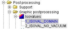
Display a prerecorded representation
With a magnetic application, to display the graphic representation of the magnetic flux density as isovalues on the entire domain :
| Step | Action |
|---|---|
| 1 |
In the data tree, point on 1_isoval_domain
|
| 2 | In the contextual menu click on Display isovalues |
Main commands
The main commands are listed in the table below.
| Command | Effect |
|---|---|
| Display isovalues | Calculation and displaying of selected isovalues: 1_isoval_domain / 1_isoval_no_vacuum / isoval_1 … |
| Hide isovalues |
Hiding active isovalues (represented in the graphic zone) |
| New isovalues |
Definition of isovalues (name, support, local quantity) + calculation and display |