Feko is a comprehensive electromagnetic solver with multiple solution methods that is used for electromagnetic field analyses
involving 3D objects of arbitrary shapes.
3D views are used to display and interact with the model. You can zoom, rotate and pan around a 3D model using the keyboard,
mouse or a combination of both. You can use a 3D mouse, specify a view or select specific parts of a model. Multiple 3D
views are supported.
Define field or current data using either far field data, near field data, spherical mode data or PCB current data. Use
the field/current definition when defining an equivalent source or a receiving antenna.
Import far field data from a Feko (.ffe), external ASCII or a CST far field scan (.ffs) file to create a far field data definition. Use the far field data when defining an equivalent source or receiving
antenna.
Import near field data from a .efe file and / or .hfe file to define a near field data aperture. Use the near field data aperture when defining an equivalent source or
receiving antenna.
Import near field data from Feko field on a Cartesian boundary (.efe and / or .hfe), Sigrity input file (.nfd), MVG measurement file (.mfxml) or a CST near field scan (.nfs) to create a near field data definition. Use the near field data definition when defining an equivalent source or
receiving antenna.
Import spherical modes data from a TICRA .sph file or import from a .sph file exported by CADFEKO, to create a spherical modes data definition. Use the spherical modes data definition when defining an equivalent
source or receiving antenna.
Define the propagation direction, index scheme and modes to create spherical modes data. Use the spherical modes data
definition when defining an equivalent source or receiving antenna.
Import printed circuit board (PCB) current data from a PollEx radiated emission interface (.rei) file to create a PCB current data definition. Use the current data definition when defining an equivalent source.
Import solution coefficient data (multi-frequency or single frequency) from a .sol file to create a solution coefficient data definition. Use the solution coefficient data definition when defining
a solution coefficient source.
Define a medium with specific material properties, import a predefined medium from the media library or add a medium from
your model to the media library.
Defined media can be applied to the model in various ways. Some media settings are applied to regions, others on faces
and wires. The rules for defining media varies between the different solution methods.
Use a periodic boundary condition (PBC) to analyse infinite periodic structures. A typical application of PBC is to
analyse frequency selective surface (FSS) structures.
Create an arbitrary finite antenna array that consists of an array of contributing elements, either with direct feeds for
each element or via indirect coupling, and solve with the efficient domain Green's function method (DGFM).
Use the windscreen tools to define a curved reference surface constrained by a cloud of points, normals and optional U′V′ parameters. The constrained surface is then used as a reference to create a work surface where windscreen layers and curved
parameterised windscreen antenna elements can be created.
Many electromagnetic compatibility and interference problems involve cables that either radiate, are irradiated or cause
coupling into other cables, devices or antennas. Use the cable modelling tool and solver to analyse the coupling and radiation.
For a frequency domain result, the electromagnetic fields and currents are calculated at a single frequency or frequency
range. When the finite difference time domain (FDTD) solver is used, the frequency must be specified to convert the native time domain results to the frequency domain.
The excitation of an antenna is normally specified as a complex voltage, but it may be useful to specify the total radiated
or source power instead. The result is then scaled to yield the desired source power level.
A port is a mathematical representation of where energy can enter (source) or leave a model (sink). Use a port
to add sources and discrete loads to a model.
Perform multiple solutions for a single model using multiple configurations. Multiple configurations remove the requirement
to create multiple models with different solution requests.
Use an infinite plane or half-space to model a ground plane efficiently. The number of triangles in the model is reduced
as the ground plane is not discretised into triangles.
Domain connectivity approach allows meshes of specific parts to be treated as if “connected” during MoM and MoM/MLFMM solutions in places where the borders of the meshes are close together, even if the mesh vertices on those borders
are not coincident.
A CADFEKO.cfm file can be imported into EDITFEKO to make use of more advanced features available in EDITFEKO and to directly edit the .pre file for more flexible solution configurations.
During the design process, the development of a model can introduce a range of issues that can lead to a non-simulation-ready
model. Use the validation toolset to verify that the model is simulation-ready or to search, detect and flag discrepancies.
The default solver used in Feko is the method of moments (MoM) - surface equivalence principle (SEP). A solver is specified per model, per face or per region, and depends on the solver in question.
CADFEKO has a collection of tools that allows you to quickly validate the model, for example, perform calculations using
a calculator, measure distances, measure angles and export images.
EDITFEKO is used to construct advanced models (both the geometry and solution requirements) using a high-level scripting language
which includes loops and conditional statements.
One of the key features in Feko is that it includes a broad set of unique and hybridised solution methods. Effective use of Feko features requires an understanding of the available methods.
Feko offers state-of-the-art optimisation engines based on generic algorithm (GA) and other methods, which can be used
to automatically optimise the design and determine the optimum solution.
Feko writes all the results to an ASCII output file .out as well as a binary output file .bof for usage by POSTFEKO. Use the .out file to obtain additional information about the solution.
CADFEKO and POSTFEKO have a powerful, fast, lightweight scripting language integrated into the application allowing you to create
models, get hold of simulation results and model configuration information as well as manipulation of data and automate
repetitive tasks.
Define field or current data using either far field data, near field data, spherical mode data or PCB current data. Use
the field/current definition when defining an equivalent source or a receiving antenna.
Import near field data from a .efe file and / or .hfe file to define a near field data aperture. Use the near field data aperture when defining an equivalent source or
receiving antenna.
Import near field data from a .efe
file and / or .hfe file to define a near
field data aperture. Use the near field data aperture when defining an equivalent source or
receiving antenna.
The .efe
and .hfe files do not contain
information regarding the coordinates system, frequency or number of points. As a
result, you need to supply the above information to define the near field data
aperture.
On the Construct tab, in the Define group, click the Field/Current Data icon. From the drop-down list
select Define Near Field Data.
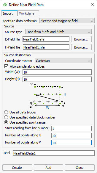
In the Aperture data definitiondrop-down list, select one of the following:
Electric and Magnetic
field
Electric field
Magnetic field
In the Source type field, select one of the
following:
Load an ASCII text file
Note: The units are V/m
for the E-field and A/m for the H-field.
Load from *.hfe file
In the E-field file field, browse to the E-field file
location.
In the H-field file field, browse to the H-field file
location
In the Coordinate system field, select one of the
following:
The physical location of the sample points and how they relate to the
defined aperture can be specified.
[Optional] Select the Also sample along edges check box
to assume the outer sample points lie on the edges of the defined
aperture.
CAUTION:
For multiple near field sources in a single model, sample
points may not lie on any two aperture edges that share a common side. This
results in two elementary dipoles with the same location and polarisation to
be included, leading to incorrect results.
For options Cylindrical or Spherical, select the Swap source and field
validity regions check box if the fields on the inside of the
region are equivalent to the calculated field values.
In the Width (W) field, specify the aperture
width.
In the Height (H) field, specify the aperture
height.
Select one of the following:
To select near field data from multi-frequency .efe and .hfe files, select Use all
data blocks. The data is interpolated for use at the
operating frequency.
To select near field data at a specific frequency in .efe and .hfe files, select Use
specified data block number and enter the number of the
relevant data block.
To select a specific near field pattern in .efe and .hfe files, select Use
specified point range1.
In the Start reading from line number field,
specify the first line number to be read in the file.
Note: Comment
lines and empty lines are not counted.
For example, a
file with 100 points per near field, the second block starts
reading from line 101, regardless of any comment lines.
In the Number of points along U field,
specify the number of points along the U axis.
In the Number of points along V field,
specify the number of points along the V axis.
In the Label field, specify a unique label for the near
field data.
Click Create to define the near field data and to
close the dialog.
1 Near field patterns are typically
frequency-dependent and models with radiation pattern sources usually
have only a single solution frequency. If the radiation pattern is
calculated using a frequency sweep in Feko,
the .efe and
.hfe files
contain multiple patterns.