vrptc
Vehicle routing problem with time constraints.
Attention: Valid only with Altair Advanced Optimization
Extension
Syntax
[CarsUsed,Petals,PetalTime,PetalCost,totalCost] = vrptc(T, D, CA, CC, loadTime, workTime)
[CarsUsed,Petals,PetalTime,PetalCost,totalCost] = vrptc(T, D, CA, CC, loadTime, workTime, options)
Inputs
- T
- A time matrix such that T(i,j) is the travel time from site i to site j. Site 1 is the common depot from which all vehicles begin their tours, and the other sites are for the N customers.
- D
- A distance matrix such that D(i,j) is the distance from site i to site j.
- CA
- The car availabilities, a vector containing the number of vehicles of each of M types in the fleet.
- CC
- The car costs, either a vector or a matrix containing the cost of each vehicle type.
- loadTime
- The time to load or unload a vehicle at a customer site.
- workTime
- The maximum working time for any vehicle.
- options
- A struct containing the genetic algorithm option settings.
Outputs
- CarsUsed
- A vector containing the type of each vehicle used.
- Petals
- A column vector of cells, with a cell for each vehicle used. Each cell is a petal, a row vector of customer indices traversed by that vehicle.
- PetalTime
- A vector containing the working time for each vehicle used.
- PetalCost
- A vector containing the travel cost for each vehicle used, including a return to the depot.
- totalCost
- The total cost to cover the path distances.
Examples
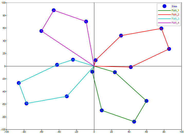
Find a set of paths through the following customer locations map for a maximum of four vehicles, each of which can work for at most 60 minutes.
% create customer site list, transposing locations from columns to rows
custsites = [77, -60, -86,  24,  46, -9,   9, 2, 42, -31, -77, -24,  60, 31, 86, -2, -42, -46;
             59,  55, -27, -10, -88, 70, -70, 9, -2, -48, -59,  10, -55, 48, 27, -9,   2,  88].';
depot = [0, 0];

% create distance matrix
numcus = size(custsites, 1);
numdim = numcus + 1;
D = zeros(numdim);

for jj = 2:numdim	% depot to site distances
	s2 = custsites(jj-1,:);
	D(1,jj) = norm(s2-depot);
	D(jj,1) = D(1,jj);
end

for ii = 2:numdim	% site to site distances
	s1 = custsites(ii-1,:);

	for jj = ii:numdim
		s2 = custsites(jj-1,:);
		D(ii,jj) = norm(s2-s1);
		D(jj,ii) = D(ii,jj);
	end
end

% find solution
T = D / 60;
CA = 4;
CC = 1;
loadTime = 10;
workTime = 60;
options = gaoptimset('Seed', 2021);

[CarsUsed,Petals,PetalTime,PetalCost,TotalCost] = vrptc(T, D, CA, CC, loadTime, workTime, options)

% plot
scatter(custsites(:,1), custsites(:,2), 'ob', 'markersize', 4);
hold on;
legendCell = {'Sites'};

for ii = 1:length(CarsUsed)
	n = length(Petals{ii});
	petalLoc = zeros(n+2,2);
	petalLoc(1,:) = depot;
	petalLoc([2:n+1],:) = custsites(Petals{ii},:);
	petalLoc(n+2,:) = depot;
	plot(petalLoc(:,1), petalLoc(:,2));
	legendCell{ii + 1} = strcat('Path_', num2str(ii));
end

legend(legendCell);
CarsUsed = [Matrix] 1 x 4
1 1 1 1
Petals =
{
[1,1] [Matrix] 1 x 5
16 7 5 13 4
[2,1] [Matrix] 1 x 5
9 15 1 14 8
[3,1] [Matrix] 1 x 5
12 17 3 11 10
[4,1] [Matrix] 1 x 3
6 18 2
}
PetalTime = [Matrix] 1 x 4
53.86374 53.88505 53.93456 33.81605
PetalCost = [Matrix] 1 x 4
231.82451 233.10327 236.07362 228.96328
TotalCost = 929.964679
The function is implemented as a genetic algorithm. The gaoptimset options and defaults are as follows:
- Generations: 100
- PopulationSize: 6
- Seed: 0
Larger numbers of generations and population size allow the search to proceed longer.
A non-zero seed will make the result repeatable.