Generation of Clutter / Land Usage Data
A clutter table specifies the height and attenuation for the clutter database.
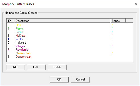
Clutter Tables
| Class ID | Name | Additional Attenuation [dB] | Mean Height [m] | ... |
|---|---|---|---|---|
| 1 | Water | 5 | 0 | ... |
| 2 | Street | 3 | 0 | ... |
| 3 | Forest | 7 | 7 | ... |
| ... | ... | ... | ... | ... |
To edit the properties of the class, open the Morpho/Clutter Class Properties dialog (click .
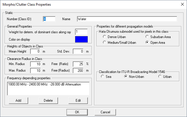
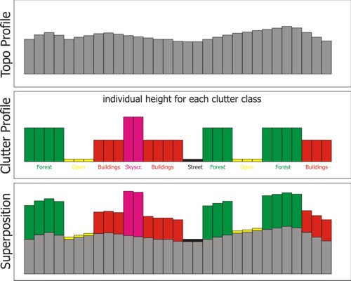
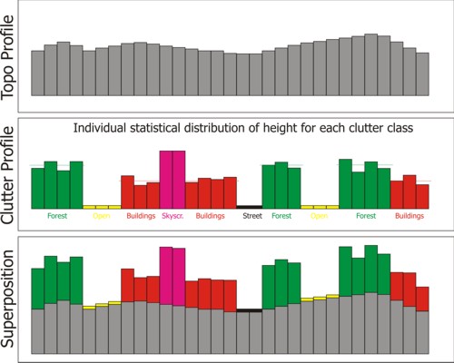
The Morpho/Clutter Class Properties dialog allows you to edit properties of the class. The meanings of ID (number) and name are obvious. The color definition is used to display the class with the defined color on the display. The height of objects (for example, forest, buildings) can be defined for each clutter class separately either as a fixed value, which applies for the whole clutter class or as a mean value with an additional standard deviation. In the second case, the clutter heights are statistically distributed to obtain a more realistic database.
The clearance, for example, the distance between the objects, can be defined individually for each clutter class. This value can be specified either as a fixed number or as a statistically distributed parameter.
- Min. Radius
- Max. Radius
- Free (Ratio)
- Free (Radius)
In the example of buildings in an urban area, this leaves something to be desired: when looking down a street one observes, in that direction, a much larger clearance value. This can be considered by defining a nonzero Free (Ratio), for example, 25% and the corresponding Free (Radius), for example, 200m. In this case with a probability of 25% a clearance of 200m is considered, while in the other 75% the clearance is equally distributed between the defined min. and max. values.
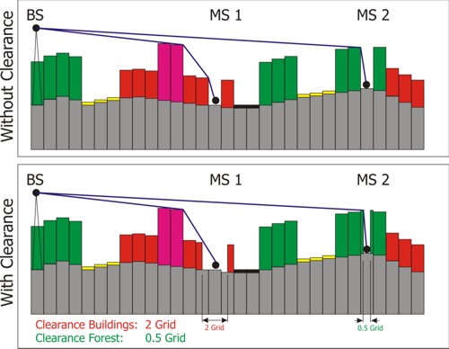
Depending on the clearance radii of the clutter classes some rays between transmitter and receiver location are diffracted at obstacles, whereas others hit the prediction plane without being diffracted. These diffraction losses, which attenuate the propagation paths additionally, can be considered by using the knife edge diffraction extension on top of the selected wave propagation model.
Most propagation tools only consider the class at the receiver pixel for the influence on the wave propagation. But this means, that if 90% of the distance between transmitter and receiver is, for example, in the clutter class urban and only the receiver pixel is in the class forest, the properties of the class forest would be used. This is not correct if 90% of the area between transmitter and receiver are urban. WinProp offers optionally the determination of the dominant class between transmitter and receiver and this class is then used for the evaluation of the receiver pixel. But some classes have a greater influence on the propagation than others. Each class can be assigned a weight factor. The higher the weight factor, the stronger the influence of the class on the propagation.
- If one urban class has a weight of one (1 class * 1 weight = 1) and the three water classes also have a weight of one (3 classes * 1 weight = 3), the dominant class is water.
- If one urban class has a weight of five (1 class * 5 weight = 5 ) and the three water classes have a weight of one (3 classes * 1 weight = 3), the dominant class is urban.
- dense urban
- medium urban
- suburban
- open area
The same sub-model can be used for the whole prediction area, although this is not always a good solution when the area is not homogeneous.
WinProp offers the option, to use for each clutter class
a different sub-model of the Hata-Okumura model. For example, for the clutter class
agricultural area
the sub-model Open Area could be
used while for the clutter class city center
the sub-model Dense
Urban could be used. This increases the accuracy of the
prediction.
- The frequency bands defined for a clutter class must not overlap.
- The frequency bands can be defined individually for each clutter class
- For class 1, the frequency bands can be 300 MHz to 1000 MHz and 1000 MHz to 2000 MHz.
- For class 2, the frequency bands can be 300 MHz to 700 MHz, 700 MHz to 1200 MHz and 1200 MHz to 2000 MHz.
- If a frequency used for a transmitter is not included in one of the frequency bands of the clutter class, the propagation is not computed for this pixel. Frequency bands can be added, deleted or edited with the three buttons below the list of frequency bands.
The properties of a frequency band can be defined with the following dialog:
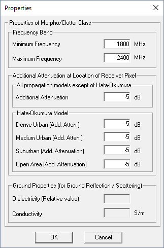
The band of frequencies is defined in the upper part of the dialog. For all propagation models, except Hata-Okumura (for example, two-ray model, parabolic equations), an additional attenuation can be defined which is added to all receiver pixels at this location. The Hata-Okumura model contains four sub-models, and therefore the additional attenuation can be defined for each sub-model individually. Depending on the model which is currently selected, the appropriate loss is selected.
For the parabolic equation model (PE) and the 3D scatting option, the electromagnetic properties of the ground can be defined. These values are used to determine the reflection/scattering loss of the waves reflected/scattered at the ground (the relative permeability is always assumed to be 1.0).