Seam Weld Fatigue

The seam weld fatigue implemented in SimSolid is based on linearization of stress in the conjunction with Volvo method and following that it predicts fatigue damage and life. Linearized stress decomposes a through-thickness elastic stress field into equivalent membrane and bending.

This method determines the contribution of bending to the total stress, and from this determines whether the weld is essentially stiff or flexible. The method typically requires two S-N curves. One is a bending S-N curve which is dominated by bending stress, and the other is a membrane S-N curve which dominated by membrane stress. Interpolation is made between the bending and membrane SN curves based on the degree of bending.

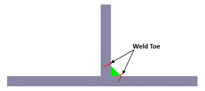
Predicted or likely failure (fatigue crack) locations at the weld toe are marked. These are the locations where the fatigue damage will be evaluated.


Figure 1. Fillet weld cross-section showing likely failure locations

Weld Stress Calculations

The seam weld fatigue damage calculation in SimSolid uses a structural stress at the location of interest using the stress linearization method (link to SimSolid linearized stress documentation) and the bending ratio associated with that stress. Linearized 
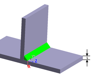
stresses are obtained in a local coordinate system along the stress linearization segment. The local coordinate system is based on the start and end points of the segment as shown in Figure 2. The X-axis of the system is along the segment from entry to exit points. The other two axes are calculated as follows:
  • If the local X-axis is not parallel to the global Y-axis:(1)
    Z l o c a l = X l o c a l * Y g l o b a l Y l o c a l = Z l o c a l * X l o c a l MathType@MTEF@5@5@+= feaahqart1ev3aaatCvAUfeBSjuyZL2yd9gzLbvyNv2CaerbuLwBLn hiov2DGi1BTfMBaeXatLxBI9gBaerbd9wDYLwzYbItLDharqqtubsr 4rNCHbGeaGqiVu0Je9sqqrpepC0xbbL8F4rqqrFfpeea0xe9Lq=Jc9 vqaqpepm0xbba9pwe9Q8fs0=yqaqpepae9pg0FirpepeKkFr0xfr=x fr=xb9adbaqaaeGaciGaaiaabeqaamaabaabaaGceaqabeaacaWGAb WaaSbaaSqaaiaadYgacaWGVbGaam4yaiaadggacaWGSbaabeaakiab g2da9iaadIfadaWgaaWcbaGaamiBaiaad+gacaWGJbGaamyyaiaadY gaaeqaaOGaaiOkaiaadMfadaWgaaWcbaGaam4zaiaadYgacaWGVbGa amOyaiaadggacaWGSbaabeaaaOqaaiaadMfadaWgaaWcbaGaamiBai aad+gacaWGJbGaamyyaiaadYgaaeqaaOGaeyypa0JaamOwamaaBaaa leaacaWGSbGaam4BaiaadogacaWGHbGaamiBaaqabaGccaGGQaGaam iwamaaBaaaleaacaWGSbGaam4BaiaadogacaWGHbGaamiBaaqabaaa aaa@5C93@
  • If the local X-axis is parallel to the global Y-axis:
    Local Y-axis ( Y l o c a l MathType@MTEF@5@5@+= feaahqart1ev3aaatCvAUfeBSjuyZL2yd9gzLbvyNv2CaerbuLwBLn hiov2DGi1BTfMBaeXatLxBI9gBaerbd9wDYLwzYbItLDharqqtubsr 4rNCHbGeaGqiVu0Je9sqqrpepC0xbbL8F4rqqrFfpeea0xe9Lq=Jc9 vqaqpepm0xbba9pwe9Q8fs0=yqaqpepae9pg0FirpepeKkFr0xfr=x fr=xb9adbaqaaeGaciGaaiaabeqaamaabaabaaGcbaGaamywamaaBa aaleaacaWGSbGaam4BaiaadogacaWGHbGaamiBaaqabaaaaa@3BA1@ ) is negative of global-X if local-X is along positive global-Y, and vice versa.(2)
    Z l o c a l = X l o c a l * Y l o c a l MathType@MTEF@5@5@+= feaahqart1ev3aaatCvAUfeBSjuyZL2yd9gzLbvyNv2CaerbuLwBLn hiov2DGi1BTfMBaeXatLxBI9gBaerbd9wDYLwzYbItLDharqqtubsr 4rNCHbGeaGqiVu0Je9sqqrpepC0xbbL8F4rqqrFfpeea0xe9Lq=Jc9 vqaqpepm0xbba9pwe9Q8fs0=yqaqpepae9pg0FirpepeKkFr0xfr=x fr=xb9adbaqaaeGaciGaaiaabeqaamaabaabaaGcbaGaamOwamaaBa aaleaacaWGSbGaam4BaiaadogacaWGHbGaamiBaaqabaGccqGH9aqp caWGybWaaSbaaSqaaiaadYgacaWGVbGaam4yaiaadggacaWGSbaabe aakiaacQcacaWGzbWaaSbaaSqaaiaadYgacaWGVbGaam4yaiaadgga caWGSbaabeaaaaa@48C5@


Figure 2.
From the extracted stress values above, the average membrane stress tensor plus the ending bending stress tensors at the entry and exit points are calculated using numerical integration.(3)
σ i m = 1 T T / 2 T / 2 σ i d x MathType@MTEF@5@5@+= feaahqart1ev3aaatCvAUfeBSjuyZL2yd9gzLbvyNv2CaerbuLwBLn hiov2DGi1BTfMBaeXatLxBI9gBaerbd9wDYLwzYbItLDharqqtubsr 4rNCHbGeaGqiVu0Je9sqqrpepC0xbbL8F4rqqrFfpeea0xe9Lq=Jc9 vqaqpepm0xbba9pwe9Q8fs0=yqaqpepae9pg0FirpepeKkFr0xfr=x fr=xb9adbaqaaeGaciGaaiaabeqaamaabaabaaGcbaGaeq4Wdm3aa0 baaSqaaiaadMgaaeaacaWGTbaaaOGaeyypa0ZaaSaaaeaacaaIXaaa baGaamivaaaadaWdbaqaamaaDaaaleaacqGHsislcaWGubGaai4lai aaikdaaeaacaWGubGaai4laiaaikdaaaGccqaHdpWCdaWgaaWcbaGa amyAaaqabaGccaWGKbGaamiEaaWcbeqab0Gaey4kIipaaaa@48F3@
(4)
σ i S b = 6 T 2 T / 2 T / 2 σ i x d x MathType@MTEF@5@5@+= feaahqart1ev3aaatCvAUfeBSjuyZL2yd9gzLbvyNv2CaerbuLwBLn hiov2DGi1BTfMBaeXatLxBI9gBaerbd9wDYLwzYbItLDharqqtubsr 4rNCHbGeaGqiVu0Je9sqqrpepC0xbbL8F4rqqrFfpeea0xe9Lq=Jc9 vqaqpepm0xbba9pwe9Q8fs0=yqaqpepae9pg0FirpepeKkFr0xfr=x fr=xb9adbaqaaeGaciGaaiaabeqaamaabaabaaGcbaGaeq4Wdm3aa0 baaSqaaiaadMgacaWGtbaabaGaamOyaaaakiabg2da9iabgkHiTmaa laaabaGaaGOnaaqaaiaadsfadaahaaWcbeqaaiaaikdaaaaaaOWaa8 qaaeaadaqhaaWcbaGaeyOeI0Iaamivaiaac+cacaaIYaaabaGaamiv aiaac+cacaaIYaaaaOGaeq4Wdm3aaSbaaSqaaiaadMgaaeqaaOGaam iEaiaadsgacaWG4baaleqabeqdcqGHRiI8aaaa@4CA2@
(5)
σ i E b = σ i S b MathType@MTEF@5@5@+= feaahqart1ev3aaatCvAUfeBSjuyZL2yd9gzLbvyNv2CaerbuLwBLn hiov2DGi1BTfMBaeXatLxBI9gBaerbd9wDYLwzYbItLDharqqtubsr 4rNCHbGeaGqiVu0Je9sqqrpepC0xbbL8F4rqqrFfpeea0xe9Lq=Jc9 vqaqpepm0xbba9pwe9Q8fs0=yqaqpepae9pg0FirpepeKkFr0xfr=x fr=xb9adbaqaaeGaciGaaiaabeqaamaabaabaaGcbaGaeq4Wdm3aa0 baaSqaaiaadMgacaWGfbaabaGaamOyaaaakiabg2da9iabgkHiTiab eo8aZnaaDaaaleaacaWGPbGaam4uaaqaaiaadkgaaaaaaa@411C@
Where,
  • σ i m MathType@MTEF@5@5@+= feaahqart1ev3aaatCvAUfeBSjuyZL2yd9gzLbvyNv2CaerbuLwBLn hiov2DGi1BTfMBaeXatLxBI9gBaerbd9wDYLwzYbItLDharqqtubsr 4rNCHbGeaGqiVu0Je9sqqrpepC0xbbL8F4rqqrFfpeea0xe9Lq=Jc9 vqaqpepm0xbba9pwe9Q8fs0=yqaqpepae9pg0FirpepeKkFr0xfr=x fr=xb9adbaqaaeGaciGaaiaabeqaamaabaabaaGcbaGaeq4Wdm3aa0 baaSqaaiaadMgaaeaacaWGTbaaaaaa@39C3@ is equal to the i t h MathType@MTEF@5@5@+= feaahqart1ev3aaatCvAUfeBSjuyZL2yd9gzLbvyNv2CaerbuLwBLn hiov2DGi1BTfMBaeXatLxBI9gBaerbd9wDYLwzYbItLDharqqtubsr 4rNCHbGeaGqiVu0Je9sqqrpepC0xbbL8F4rqqrFfpeea0xe9Lq=Jc9 vqaqpepm0xbba9pwe9Q8fs0=yqaqpepae9pg0FirpepeKkFr0xfr=x fr=xb9adbaqaaeGaciGaaiaabeqaamaabaabaaGcbaGaamyAamaaCa aaleqabaGaamiDaiaadIgaaaaaaa@38F4@ component of membrane stress.
  • σ i MathType@MTEF@5@5@+= feaahqart1ev3aaatCvAUfeBSjuyZL2yd9gzLbvyNv2CaerbuLwBLn hiov2DGi1BTfMBaeXatLxBI9gBaerbd9wDYLwzYbItLDharqqtubsr 4rNCHbGeaGqiVu0Je9sqqrpepC0xbbL8F4rqqrFfpeea0xe9Lq=Jc9 vqaqpepm0xbba9pwe9Q8fs0=yqaqpepae9pg0FirpepeKkFr0xfr=x fr=xb9adbaqaaeGaciGaaiaabeqaamaabaabaaGcbaGaeq4Wdm3aaS baaSqaaiaadMgaaeqaaaaa@38D0@ is equal to the i t h MathType@MTEF@5@5@+= feaahqart1ev3aaatCvAUfeBSjuyZL2yd9gzLbvyNv2CaerbuLwBLn hiov2DGi1BTfMBaeXatLxBI9gBaerbd9wDYLwzYbItLDharqqtubsr 4rNCHbGeaGqiVu0Je9sqqrpepC0xbbL8F4rqqrFfpeea0xe9Lq=Jc9 vqaqpepm0xbba9pwe9Q8fs0=yqaqpepae9pg0FirpepeKkFr0xfr=x fr=xb9adbaqaaeGaciGaaiaabeqaamaabaabaaGcbaGaamyAamaaCa aaleqabaGaamiDaiaadIgaaaaaaa@38F4@ component of extracted stress value.
  • σ i S b MathType@MTEF@5@5@+= feaahqart1ev3aaatCvAUfeBSjuyZL2yd9gzLbvyNv2CaerbuLwBLn hiov2DGi1BTfMBaeXatLxBI9gBaerbd9wDYLwzYbItLDharqqtubsr 4rNCHbGeaGqiVu0Je9sqqrpepC0xbbL8F4rqqrFfpeea0xe9Lq=Jc9 vqaqpepm0xbba9pwe9Q8fs0=yqaqpepae9pg0FirpepeKkFr0xfr=x fr=xb9adbaqaaeGaciGaaiaabeqaamaabaabaaGcbaGaeq4Wdm3aa0 baaSqaaiaadMgacaWGtbaabaGaamOyaaaaaaa@3A90@ is equal to the i t h MathType@MTEF@5@5@+= feaahqart1ev3aaatCvAUfeBSjuyZL2yd9gzLbvyNv2CaerbuLwBLn hiov2DGi1BTfMBaeXatLxBI9gBaerbd9wDYLwzYbItLDharqqtubsr 4rNCHbGeaGqiVu0Je9sqqrpepC0xbbL8F4rqqrFfpeea0xe9Lq=Jc9 vqaqpepm0xbba9pwe9Q8fs0=yqaqpepae9pg0FirpepeKkFr0xfr=x fr=xb9adbaqaaeGaciGaaiaabeqaamaabaabaaGcbaGaamyAamaaCa aaleqabaGaamiDaiaadIgaaaaaaa@38F4@ component of bending stress at the entry.
  • σ i E b MathType@MTEF@5@5@+= feaahqart1ev3aaatCvAUfeBSjuyZL2yd9gzLbvyNv2CaerbuLwBLn hiov2DGi1BTfMBaeXatLxBI9gBaerbd9wDYLwzYbItLDharqqtubsr 4rNCHbGeaGqiVu0Je9sqqrpepC0xbbL8F4rqqrFfpeea0xe9Lq=Jc9 vqaqpepm0xbba9pwe9Q8fs0=yqaqpepae9pg0FirpepeKkFr0xfr=x fr=xb9adbaqaaeGaciGaaiaabeqaamaabaabaaGcbaGaeq4Wdm3aa0 baaSqaaiaadMgacaWGfbaabaGaamOyaaaaaaa@3A82@ is equal to the i t h MathType@MTEF@5@5@+= feaahqart1ev3aaatCvAUfeBSjuyZL2yd9gzLbvyNv2CaerbuLwBLn hiov2DGi1BTfMBaeXatLxBI9gBaerbd9wDYLwzYbItLDharqqtubsr 4rNCHbGeaGqiVu0Je9sqqrpepC0xbbL8F4rqqrFfpeea0xe9Lq=Jc9 vqaqpepm0xbba9pwe9Q8fs0=yqaqpepae9pg0FirpepeKkFr0xfr=x fr=xb9adbaqaaeGaciGaaiaabeqaamaabaabaaGcbaGaamyAamaaCa aaleqabaGaamiDaiaadIgaaaaaaa@38F4@ component of bending stress at the exit.
  • L MathType@MTEF@5@5@+= feaahqart1ev3aaatCvAUfeBSjuyZL2yd9gzLbvyNv2CaerbuLwBLn hiov2DGi1BTfMBaeXatLxBI9gBaerbd9wDYLwzYbItLDharqqtubsr 4rNCHbGeaGqiVu0Je9sqqrpepC0xbbL8F4rqqrFfpeea0xe9Lq=Jc9 vqaqpepm0xbba9pwe9Q8fs0=yqaqpepae9pg0FirpepeKkFr0xfr=x fr=xb9adbaqaaeGaciGaaiaabeqaamaabaabaaGcbaGaamitaaaa@36C4@ is equal to the i t h MathType@MTEF@5@5@+= feaahqart1ev3aaatCvAUfeBSjuyZL2yd9gzLbvyNv2CaerbuLwBLn hiov2DGi1BTfMBaeXatLxBI9gBaerbd9wDYLwzYbItLDharqqtubsr 4rNCHbGeaGqiVu0Je9sqqrpepC0xbbL8F4rqqrFfpeea0xe9Lq=Jc9 vqaqpepm0xbba9pwe9Q8fs0=yqaqpepae9pg0FirpepeKkFr0xfr=x fr=xb9adbaqaaeGaciGaaiaabeqaamaabaabaaGcbaGaamyAamaaCa aaleqabaGaamiDaiaadIgaaaaaaa@38F4@ Length of the stress linearization segment.
  • x MathType@MTEF@5@5@+= feaahqart1ev3aaatCvAUfeBSjuyZL2yd9gzLbvyNv2CaerbuLwBLn hiov2DGi1BTfMBaeXatLxBI9gBaerbd9wDYLwzYbItLDharqqtubsr 4rNCHbGeaGqiVu0Je9sqqrpepC0xbbL8F4rqqrFfpeea0xe9Lq=Jc9 vqaqpepm0xbba9pwe9Q8fs0=yqaqpepae9pg0FirpepeKkFr0xfr=x fr=xb9adbaqaaeGaciGaaiaabeqaamaabaabaaGcbaGaamiEaaaa@36F0@ is equal to the position of a point along the segment.
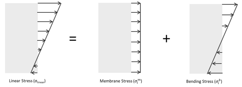
The stress quantity used for the seam weld damage parameter is the sum of the membrane and bending stresses.


Figure 3.
Hence, the stress at the top and the bottom surface is derived from the below equations:(6)
σ t o p = σ i m + σ i S b MathType@MTEF@5@5@+= feaahqart1ev3aaatCvAUfeBSjuyZL2yd9gzLbvyNv2CaerbuLwBLn hiov2DGi1BTfMBaeXatLxBI9gBaerbd9wDYLwzYbItLDharqqtubsr 4rNCHbGeaGqiVu0Je9sqqrpepC0xbbL8F4rqqrFfpeea0xe9Lq=Jc9 vqaqpepm0xbba9pwe9Q8fs0=yqaqpepae9pg0FirpepeKkFr0xfr=x fr=xb9adbaqaaeGaciGaaiaabeqaamaabaabaaGcbaGaeq4Wdm3aaS baaSqaaiaadshacaWGVbGaamiCaaqabaGccqGH9aqpcqaHdpWCdaqh aaWcbaGaamyAaaqaaiaad2gaaaGccqGHRaWkcqaHdpWCdaqhaaWcba GaamyAaiaadofaaeaacaWGIbaaaaaa@452D@
(7)
σ bottom = σ i m σ iS b (since  σ iE b = σ iS b ) MathType@MTEF@5@5@+= feaahqart1ev3aaatCvAUfeBSjuyZL2yd9gzLbvyNv2CaerbuLwBLn hiov2DGi1BTfMBaeXatLxBI9gBaerbd9wDYLwzYbItLDharqqtubsr 4rNCHbGeaGqiVu0Je9sqqrpepC0xbbL8F4rqqrFfpeea0xe9Lq=Jc9 vqaqpepm0xbba9pwe9Q8fs0=yqaqpepae9pg0FirpepeKkFr0xfr=x fr=xb9adbaqaaeGaciGaaiaabeqaamaabaabaaGcbaGaeq4Wdm3aaS baaSqaaiaadkgacaWGVbGaamiDaiaadshacaWGVbGaamyBaaqabaGc cqGH9aqpcqaHdpWCdaqhaaWcbaGaamyAaaqaaiaad2gaaaGccqGHsi slcqaHdpWCdaqhaaWcbaGaamyAaiaadofaaeaacaWGIbaaaOGaaiik aiaabohacaqGPbGaaeOBaiaabogacaqGLbGaaeiiaiabeo8aZnaaDa aaleaacaWGPbGaamyraaqaaiaadkgaaaGccqGH9aqpcqGHsislcqaH dpWCdaqhaaWcbaGaamyAaiaadofaaeaacaWGIbaaaOGaaiykaaaa@59E3@
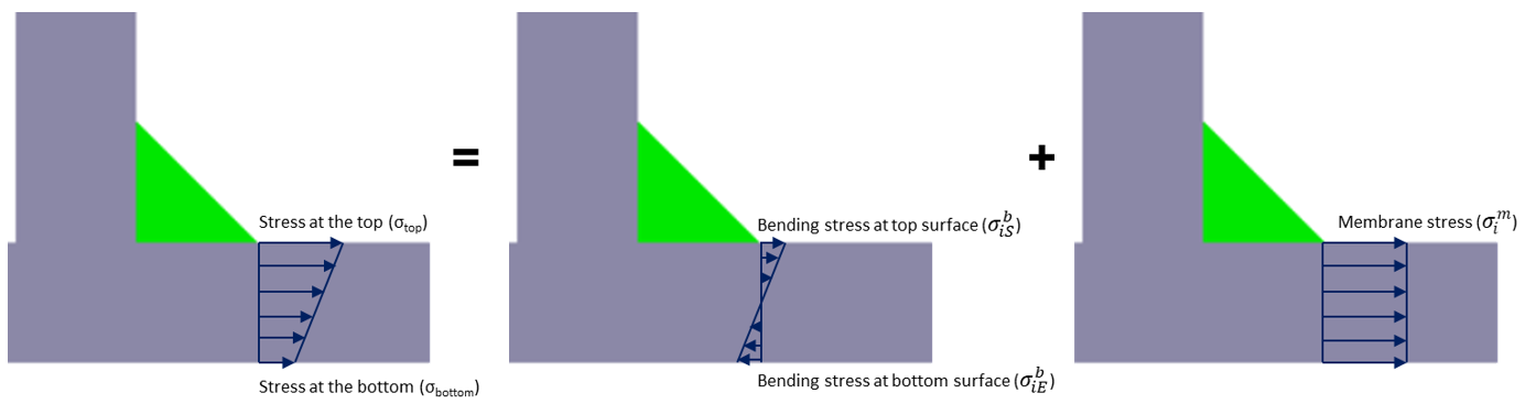
Note: Therefore, the calculation method used in the seam weld analysis engine is equally applicable to stresses calculated from either solid or thin-shell models. This generates top and bottom surface stresses in the same form as would be generated from a thin-shell model.


Figure 4.

Bending Ratio (r)

Experiments show that two types of SN curves are required to perform seam weld fatigue analysis based on a method suggested by M. Fermér, M Andréasson, and B 
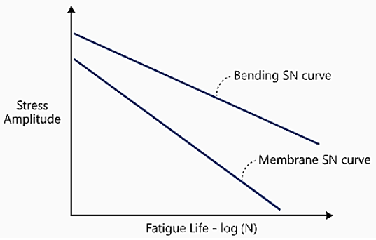
Frodin. Based on lab tests, two SN curves were plotted (Figure 5). The upper curve is obtained in tests where the maximum stress is dominated by bending moment and the lower curve is obtained from tests where membrane force dominates the maximum stress.


Figure 5.
The upper and lower curves are referred to as bending S-N curve and membrane S-N curve, respectively. It is recommended that membrane S-N curve should be used when membrane stress dominates in an element and a bending S-N curve should be used when bending stress dominates. Interpolation between the two curves may be carried out depending on the degree of bending dominance.(8)
r = σ i b σ i b + σ i m MathType@MTEF@5@5@+= feaahqart1ev3aaatCvAUfeBSjuyZL2yd9gzLbvyNv2CaerbuLwBLn hiov2DGi1BTfMBaeXatLxBI9gBaerbd9wDYLwzYbItLDharqqtubsr 4rNCHbGeaGqiVu0Je9sqqrpepC0xbbL8F4rqqrFfpeea0xe9Lq=Jc9 vqaqpepm0xbba9pwe9Q8fs0=yqaqpepae9pg0FirpepeKkFr0xfr=x fr=xb9adbaqaaeGaciGaaiaabeqaamaabaabaaGcbaGaamOCaiabg2 da9maalaaabaWaaqWaaeaacqaHdpWCdaqhaaWcbaGaamyAaaqaaiaa dkgaaaaakiaawEa7caGLiWoaaeaadaabdaqaaiabeo8aZnaaDaaale aacaWGPbaabaGaamOyaaaaaOGaay5bSlaawIa7aiabgUcaRmaaemaa baGaeq4Wdm3aa0baaSqaaiaadMgaaeaacaWGTbaaaaGccaGLhWUaay jcSdaaaaaa@4DC0@
Where,
  • σ i b MathType@MTEF@5@5@+= feaahqart1ev3aaatCvAUfeBSjuyZL2yd9gzLbvyNv2CaerbuLwBLn hiov2DGi1BTfMBaeXatLxBI9gBaerbd9wDYLwzYbItLDharqqtubsr 4rNCHbGeaGqiVu0Je9sqqrpepC0xbbL8F4rqqrFfpeea0xe9Lq=Jc9 vqaqpepm0xbba9pwe9Q8fs0=yqaqpepae9pg0FirpepeKkFr0xfr=x fr=xb9adbaqaaeGaciGaaiaabeqaamaabaabaaGcbaGaeq4Wdm3aa0 baaSqaaiaadMgaaeaacaWGIbaaaaaa@39B8@ is the maximum bending stress equal to 6 T 2 T / 2 T / 2 σ i x d x MathType@MTEF@5@5@+= feaahqart1ev3aaatCvAUfeBSjuyZL2yd9gzLbvyNv2CaerbuLwBLn hiov2DGi1BTfMBaeXatLxBI9gBaerbd9wDYLwzYbItLDharqqtubsr 4rNCHbGeaGqiVu0Je9sqqrpepC0xbbL8F4rqqrFfpeea0xe9Lq=Jc9 vqaqpepm0xbba9pwe9Q8fs0=yqaqpepae9pg0FirpepeKkFr0xfr=x fr=xb9adbaqaaeGaciGaaiaabeqaamaabaabaaGcbaWaaSaaaeaaca aI2aaabaGaamivamaaCaaaleqabaGaaGOmaaaaaaGcdaWdbaqaamaa DaaaleaacqGHsislcaWGubGaai4laiaaikdaaeaacaWGubGaai4lai aaikdaaaaabeqab0Gaey4kIipakiabeo8aZnaaBaaaleaacaWGPbaa beaakiaadIhacaWGKbGaamiEaaaa@45FD@ .
  • σ i m MathType@MTEF@5@5@+= feaahqart1ev3aaatCvAUfeBSjuyZL2yd9gzLbvyNv2CaerbuLwBLn hiov2DGi1BTfMBaeXatLxBI9gBaerbd9wDYLwzYbItLDharqqtubsr 4rNCHbGeaGqiVu0Je9sqqrpepC0xbbL8F4rqqrFfpeea0xe9Lq=Jc9 vqaqpepm0xbba9pwe9Q8fs0=yqaqpepae9pg0FirpepeKkFr0xfr=x fr=xb9adbaqaaeGaciGaaiaabeqaamaabaabaaGcbaGaeq4Wdm3aa0 baaSqaaiaadMgaaeaacaWGTbaaaaaa@39C3@ is the maximum membrane stress equal to 1 T T / 2 T / 2 σ i d x MathType@MTEF@5@5@+= feaahqart1ev3aaatCvAUfeBSjuyZL2yd9gzLbvyNv2CaerbuLwBLn hiov2DGi1BTfMBaeXatLxBI9gBaerbd9wDYLwzYbItLDharqqtubsr 4rNCHbGeaGqiVu0Je9sqqrpepC0xbbL8F4rqqrFfpeea0xe9Lq=Jc9 vqaqpepm0xbba9pwe9Q8fs0=yqaqpepae9pg0FirpepeKkFr0xfr=x fr=xb9adbaqaaeGaciGaaiaabeqaamaabaabaaGcbaWaaSaaaeaaca aIXaaabaGaamivaaaadaWdbaqaamaaDaaaleaacqGHsislcaWGubGa ai4laiaaikdaaeaacaWGubGaai4laiaaikdaaaaabeqab0Gaey4kIi pakiabeo8aZnaaBaaaleaacaWGPbaabeaakiaadsgacaWG4baaaa@4408@
The average bending ratio, ( r b A V G ) MathType@MTEF@5@5@+= feaahqart1ev3aaatCvAUfeBSjuyZL2yd9gzLbvyNv2CaerbuLwBLn hiov2DGi1BTfMBaeXatLxBI9gBaerbd9wDYLwzYbItLDharqqtubsr 4rNCHbGeaGqiVu0Je9sqqrpepC0xbbL8F4rqqrFfpeea0xe9Lq=Jc9 vqaqpepm0xbba9pwe9Q8fs0=yqaqpepae9pg0FirpepeKkFr0xfr=x fr=xb9adbaqaaeGaciGaaiaabeqaamaabaabaaGcbaGaaiikaiaadk hadaqhaaWcbaGaamOyaaqaaiaadgeacaWGwbGaam4raaaakiaacMca aaa@3BCE@ , is defined as:(9)
( r b A V G ) = i = 1 n ( r σ T O P 2 i = 1 n σ T O P 2 MathType@MTEF@5@5@+= feaahqart1ev3aaatCvAUfeBSjuyZL2yd9gzLbvyNv2CaerbuLwBLn hiov2DGi1BTfMBaeXatLxBI9gBaerbd9wDYLwzYbItLDharqqtubsr 4rNCHbGeaGqiVu0Je9sqqrpepC0xbbL8F4rqqrFfpeea0xe9Lq=Jc9 vqaqpepm0xbba9pwe9Q8fs0=yqaqpepae9pg0FirpepeKkFr0xfr=x fr=xb9adbaqaaeGaciGaaiaabeqaamaabaabaaGcbaGaaiikaiaadk hadaqhaaWcbaGaamOyaaqaaiaadgeacaWGwbGaam4raaaakiaacMca cqGH9aqpdaWcaaqaaiabggHiLpaaDaaaleaacaWGPbGaeyypa0JaaG ymaaqaaiaad6gaaaGccaGGOaGaamOCamaadmaabaGaeq4Wdm3aa0ba aSqaaiaadsfacaWGpbGaamiuaaqaaiaaikdaaaaakiaawUfacaGLDb aaaeaacqGHris5daqhaaWcbaGaamyAaiabg2da9iaaigdaaeaacaWG UbaaaOWaamWaaeaacqaHdpWCdaqhaaWcbaGaamivaiaad+eacaWGqb aabaGaaGOmaaaaaOGaay5waiaaw2faaaaaaaa@57D5@
Where,
  • σ T O P 2 MathType@MTEF@5@5@+= feaahqart1ev3aaatCvAUfeBSjuyZL2yd9gzLbvyNv2CaerbuLwBLn hiov2DGi1BTfMBaeXatLxBI9gBaerbd9wDYLwzYbItLDharqqtubsr 4rNCHbGeaGqiVu0Je9sqqrpepC0xbbL8F4rqqrFfpeea0xe9Lq=Jc9 vqaqpepm0xbba9pwe9Q8fs0=yqaqpepae9pg0FirpepeKkFr0xfr=x fr=xb9adbaqaaeGaciGaaiaabeqaamaabaabaaGcbaGaeq4Wdm3aa0 baaSqaaiaadsfacaWGpbGaamiuaaqaaiaaikdaaaaaaa@3B21@ is the square of the maximum stress at the top surface when the damage is calculated, that is, at weld toe.
  • r MathType@MTEF@5@5@+= feaahqart1ev3aaatCvAUfeBSjuyZL2yd9gzLbvyNv2CaerbuLwBLn hiov2DGi1BTfMBaeXatLxBI9gBaerbd9wDYLwzYbItLDharqqtubsr 4rNCHbGeaGqiVu0Je9sqqrpepC0xbbL8F4rqqrFfpeea0xe9Lq=Jc9 vqaqpepm0xbba9pwe9Q8fs0=yqaqpepae9pg0FirpepeKkFr0xfr=x fr=xb9adbaqaaeGaciGaaiaabeqaamaabaabaaGcbaGaamOCaaaa@36EA@ is the bending ratio.

It is the weighted average of the bending ratio over all points in the loading time history.

An interpolation factor (IF) is now defined as:(10)
IF = 0.0  when  0.0 r b A V G r b T H R MathType@MTEF@5@5@+= feaahqart1ev3aaatCvAUfeBSjuyZL2yd9gzLbvyNv2CaerbuLwBLn hiov2DGi1BTfMBaeXatLxBI9gBaerbd9wDYLwzYbItLDharqqtubsr 4rNCHbGeaGqiVu0Je9sqqrpepC0xbbL8F4rqqrFfpeea0xe9Lq=Jc9 vqaqpepm0xbba9pwe9Q8fs0=yqaqpepae9pg0FirpepeKkFr0xfr=x fr=xb9adbaqaaeGaciGaaiaabeqaamaabaabaaGcbaGaaeysaiaabA eacqGH9aqpcaaIWaGaaiOlaiaaicdacaqGGaGaae4DaiaabIgacaqG LbGaaeOBaiaabccacaaIWaGaaiOlaiaaicdacqGHKjYOcaWGYbWaa0 baaSqaaiaadkgaaeaacaWGbbGaamOvaiaadEeaaaGccqGHKjYOcaWG YbWaa0baaSqaaiaadkgaaeaacaWGubGaamisaiaadkfaaaaaaa@4E52@
(11)
IF = r b A V G r b T H R 1 r b T H R  when  r b T H R < r b A V G 1.0 MathType@MTEF@5@5@+= feaahqart1ev3aaatCvAUfeBSjuyZL2yd9gzLbvyNv2CaerbuLwBLn hiov2DGi1BTfMBaeXatLxBI9gBaerbd9wDYLwzYbItLDharqqtubsr 4rNCHbGeaGqiVu0Je9sqqrpepC0xbbL8F4rqqrFfpeea0xe9Lq=Jc9 vqaqpepm0xbba9pwe9Q8fs0=yqaqpepae9pg0FirpepeKkFr0xfr=x fr=xb9adbaqaaeGaciGaaiaabeqaamaabaabaaGcbaGaaeysaiaabA eacqGH9aqpdaWcaaqaaiaadkhadaqhaaWcbaGaamOyaaqaaiaadgea caWGwbGaam4raaaakiabgkHiTiaadkhadaqhaaWcbaGaamOyaaqaai aadsfacaWGibGaamOuaaaaaOqaaiaaigdacqGHsislcaWGYbWaa0ba aSqaaiaadkgaaeaacaWGubGaamisaiaadkfaaaaaaOGaaeiiaiaabE hacaqGObGaaeyzaiaab6gacaqGGaGaamOCamaaDaaaleaacaWGIbaa baGaamivaiaadIeacaWGsbaaaOGaeyipaWJaamOCamaaDaaaleaaca WGIbaabaGaamyqaiaadAfacaWGhbaaaOGaeyizImQaaGymaiaac6ca caaIWaaaaa@5BD1@
The r b T H R MathType@MTEF@5@5@+= feaahqart1ev3aaatCvAUfeBSjuyZL2yd9gzLbvyNv2CaerbuLwBLn hiov2DGi1BTfMBaeXatLxBI9gBaerbd9wDYLwzYbItLDharqqtubsr 4rNCHbGeaGqiVu0Je9sqqrpepC0xbbL8F4rqqrFfpeea0xe9Lq=Jc9 vqaqpepm0xbba9pwe9Q8fs0=yqaqpepae9pg0FirpepeKkFr0xfr=x fr=xb9adbaqaaeGaciGaaiaabeqaamaabaabaaGcbaGaamOCamaaDa aaleaacaWGIbaabaGaamivaiaadIeacaWGsbaaaaaa@3A7B@ value is defined by the bending ratio threshold in Fatigue solution settings. It is set to 0.5 by default. If average bending ratio ( r b AVG MathType@MTEF@5@5@+= feaahqart1ev3aaatCvAUfeBSjuyZL2yd9gzLbvyNv2CaerbuLwBLn hiov2DGi1BTfMBaeXatLxBI9gBaerbd9wDYLwzYbItLDharqqtubsr 4rNCHbGeaGqiVu0Je9sqqrpepC0xbbL8F4rqqrFfpeea0xe9Lq=Jc9 vqaqpepm0xbba9pwe9Q8fs0=yqaqpepae9pg0FirpepeKkFr0xfr=x fr=xb9adbaqaaeGaciGaaiaabeqaamaabaabaaGcbaGaamOCamaaDa aaleaacaWGIbaabaGaamyqaiaadAfacaWGhbaaaaaa@3A6B@ ) is less than or equal to the bending ratio threshold ( r b THR MathType@MTEF@5@5@+= feaahqart1ev3aaatCvAUfeBSjuyZL2yd9gzLbvyNv2CaerbuLwBLn hiov2DGi1BTfMBaeXatLxBI9gBaerbd9wDYLwzYbItLDharqqtubsr 4rNCHbGeaGqiVu0Je9sqqrpepC0xbbL8F4rqqrFfpeea0xe9Lq=Jc9 vqaqpepm0xbba9pwe9Q8fs0=yqaqpepae9pg0FirpepeKkFr0xfr=x fr=xb9adbaqaaeGaciGaaiaabeqaamaabaabaaGcbaGaamOCamaaDa aaleaacaWGIbaabaGaamivaiaadIeacaWGsbaaaaaa@3A7B@ ), then the membrane S-N curve is used to assess damage. If average bending ratio is greater than the bending ratio threshold, then an S-N curve that is interpolated between membrane S-N curve and the bending S-N curve is used.

Interpolation between Membrane and Bending S-N Curves


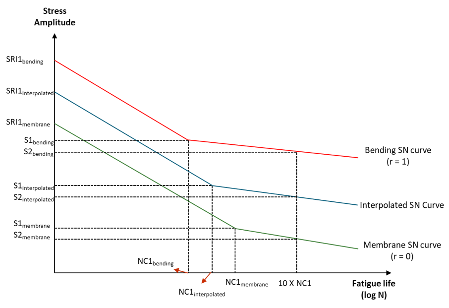
Figure 6.
The linear interpolation method, as shown in Figure 6, uses the value of the interpolation factor (IF). For the interpolated curve, the calculation is done as follows, for the Fatigue Strength coefficient value (SRI1):(12)

SRI1interpolated = SRI1membrane + (SRI1bending – SRI1membrane) ∙ IF

This defines the stress level at 1 cycle.(13)

Nc1interpolated = 10(log10Nc1membrane + (log10 Nc1bending – log10(Nc1membrane) ∙IF))

(14)

S1interpolated = S1membrane + (S1bending – S1membrane) ∙ IF

This defines the stress level at Nc1interpolated cycles. These two points define the first section of the curve up to Nc1interpolated cycles. The last section is defined by finding a third point as follows. A life value is defined being 10 times greater of the Nc1 values for the stiff and flexible curves. From these, we can calculate S2bending and S2membrane. From these, we can interpolate to get S2interpolated which defines the high cycle part of the curve.(15)

S2interpolated = S2membrane + (S2bending – S2membrane). IF

Thickness

Optionally, a thickness (size effect correction) may be applied, based on thickness t of the part. It operates as follows:

There is no effect if t T ref MathType@MTEF@5@5@+= feaahqart1ev3aaatCvAUfeBSjuyZL2yd9gzLbvyNv2CaerbuLwBLn hiov2DGi1BTfMBaeXatLxBI9gBaerbd9wDYLwzYbItLDharqqtubsr 4rNCHbGeaGqiVu0Je9sqqrpepC0xbbL8F4rqqrFfpeea0xe9Lq=Jc9 vqaqpepm0xbba9pwe9Q8fs0=yqaqpepae9pg0FirpepeKkFr0xfr=x fr=xb9adbaqaaeGaciGaaiaabeqaamaabaabaaGcbaGaamiDaiabgs MiJkaadsfadaWgaaWcbaGaamOCaiaadwgacaWGMbaabeaaaaa@3C72@ (the reference thickness or threshold can be specified in the fatigue solution settings).

The fatigue strength is reduced by a factor of T r e f t n MathType@MTEF@5@5@+= feaahqart1ev3aaatCvAUfeBSjuyZL2yd9gzLbvyNv2CaerbuLwBLn hiov2DGi1BTfMBaeXatLxBI9gBaerbd9wDYLwzYbItLDharqqtubsr 4rNCHbGeaGqiVu0Je9sqqrpepC0xbbL8F4rqqrFfpeea0xe9Lq=Jc9 vqaqpepm0xbba9pwe9Q8fs0=yqaqpepae9pg0FirpepeKkFr0xfr=x fr=xb9adbaqaaeGaciGaaiaabeqaamaabaabaaGcbaWaaeWaaeaada WcaaqaaiaadsfadaWgaaWcbaGaamOCaiaadwgacaWGMbaabeaaaOqa aiaadshaaaaacaGLOaGaayzkaaWaaWbaaSqabeaacaWGUbaaaaaa@3D80@ , where n is the thickness exponent, if t > T r e f MathType@MTEF@5@5@+= feaahqart1ev3aaatCvAUfeBSjuyZL2yd9gzLbvyNv2CaerbuLwBLn hiov2DGi1BTfMBaeXatLxBI9gBaerbd9wDYLwzYbItLDharqqtubsr 4rNCHbGeaGqiVu0Je9sqqrpepC0xbbL8F4rqqrFfpeea0xe9Lq=Jc9 vqaqpepm0xbba9pwe9Q8fs0=yqaqpepae9pg0FirpepeKkFr0xfr=x fr=xb9adbaqaaeGaciGaaiaabeqaamaabaabaaGcbaGaamiDaiabg6 da+iaadsfadaWgaaWcbaGaamOCaiaadwgacaWGMbaabeaaaaa@3BC5@ , at all lifetimes (used as a factor to up the stress).

Mean Stress Correction

FKM mean stress correction is supported for seam weld fatigue. Stress sensitivity can be defined in the fatigue solution settings dialog via the mean stress correction field. Mean stress correction for seam weld fatigue can be enabled through the seam weld fatigue solution settings dialog.

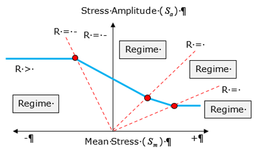
Based on FKM-Guidelines, the Haigh diagram is divided into four regimes based on the Stress ratio (R=Smin/Smax) values. The corrected value is then used to choose the SN curve for the damage and life calculation stage.

The FKM equations below illustrate the calculation of Corrected Stress Amplitude ( S e A MathType@MTEF@5@5@+= feaahqart1ev3aaatCvAUfeBSjuyZL2yd9gzLbvyNv2CaerbuLwBLn hiov2DGi1BTfMBaeXatLxBI9gBaerbd9wDYLwzYbItLDharqqtubsr 4rNCHbGeaGqiVu0Je9sqqrpepC0xbbL8F4rqqrFfpeea0xe9Lq=Jc9 vqaqpepm0xbba9pwe9Q8fs0=yqaqpepae9pg0FirpepeKkFr0xfr=x fr=xb9adbaqaaeGaciGaaiaabeqaamaabaabaaGcbaGaam4uamaaDa aaleaacaWGLbaabaGaamyqaaaaaaa@38A8@ ). The actual value of stress used in the Damage calculations is the Corrected stress Amplitude (which is 2 S e A MathType@MTEF@5@5@+= feaahqart1ev3aaatCvAUfeBSjuyZL2yd9gzLbvyNv2CaerbuLwBLn hiov2DGi1BTfMBaeXatLxBI9gBaerbd9wDYLwzYbItLDharqqtubsr 4rNCHbGeaGqiVu0Je9sqqrpepC0xbbL8F4rqqrFfpeea0xe9Lq=Jc9 vqaqpepm0xbba9pwe9Q8fs0=yqaqpepae9pg0FirpepeKkFr0xfr=x fr=xb9adbaqaaeGaciGaaiaabeqaamaabaabaaGcbaGaaGOmaiabgw SixlaadofadaqhaaWcbaGaamyzaaqaaiaadgeaaaaaaa@3BAE@ ). These equations apply for SN curves that you input.
  • Regime 1 (R>1.0): S e A = S a ( 1 M ) MathType@MTEF@5@5@+= feaahqart1ev3aaatCvAUfeBSjuyZL2yd9gzLbvyNv2CaerbuLwBLn hiov2DGi1BTfMBaeXatLxBI9gBaerbd9wDYLwzYbItLDharqqtubsr 4rNCHbGeaGqiVu0Je9sqqrpepC0xbbL8F4rqqrFfpeea0xe9Lq=Jc9 vqaqpepm0xbba9pwe9Q8fs0=yqaqpepae9pg0FirpepeKkFr0xfr=x fr=xb9adbaqaaeGaciGaaiaabeqaamaabaabaaGcbaGaam4uamaaDa aaleaacaWGLbaabaGaamyqaaaakiabg2da9iaadofadaWgaaWcbaGa amyyaaqabaGccaGGOaGaaGymaiabgkHiTiaad2eacaGGPaaaaa@3F7F@
  • Regime 2 ( R 0.0 MathType@MTEF@5@5@+= feaahqart1ev3aaatCvAUfeBSjuyZL2yd9gzLbvyNv2CaerbuLwBLn hiov2DGi1BTfMBaeXatLxBI9gBaerbd9wDYLwzYbItLDharqqtubsr 4rNCHbGeaGqiVu0Je9sqqrpepC0xbbL8F4rqqrFfpeea0xe9Lq=Jc9 vqaqpepm0xbba9pwe9Q8fs0=yqaqpepae9pg0FirpepeKkFr0xfr=x fr=xb9adbaqaaeGaciGaaiaabeqaamaabaabaaGcbaGaeyOeI0Iaey OhIuQaeyizImQaamOuaiabgsMiJkaaicdacaGGUaGaaGimaaaa@3EB8@ ): S e A = S a + M * S m MathType@MTEF@5@5@+= feaahqart1ev3aaatCvAUfeBSjuyZL2yd9gzLbvyNv2CaerbuLwBLn hiov2DGi1BTfMBaeXatLxBI9gBaerbd9wDYLwzYbItLDharqqtubsr 4rNCHbGeaGqiVu0Je9sqqrpepC0xbbL8F4rqqrFfpeea0xe9Lq=Jc9 vqaqpepm0xbba9pwe9Q8fs0=yqaqpepae9pg0FirpepeKkFr0xfr=x fr=xb9adbaqaaeGaciGaaiaabeqaamaabaabaaGcbaGaam4uamaaDa aaleaacaWGLbaabaGaamyqaaaakiabg2da9iaadofadaWgaaWcbaGa amyyaaqabaGccqGHRaWkcaWGnbGaaiOkaiaadofadaWgaaWcbaGaam yBaaqabaaaaa@4004@
  • Regime 3 (0.0<R<0.5): S e A = ( 1 + M ) S a + ( M / 3 ) * S m 1 + M / 3 MathType@MTEF@5@5@+= feaahqart1ev3aaatCvAUfeBSjuyZL2yd9gzLbvyNv2CaerbuLwBLn hiov2DGi1BTfMBaeXatLxBI9gBaerbd9wDYLwzYbItLDharqqtubsr 4rNCHbGeaGqiVu0Je9sqqrpepC0xbbL8F4rqqrFfpeea0xe9Lq=Jc9 vqaqpepm0xbba9pwe9Q8fs0=yqaqpepae9pg0FirpepeKkFr0xfr=x fr=xb9adbaqaaeGaciGaaiaabeqaamaabaabaaGcbaGaam4uamaaDa aaleaacaWGLbaabaGaamyqaaaakiabg2da9iaacIcacaaIXaGaey4k aSIaamytaiaacMcadaWcaaqaaiaadofadaWgaaWcbaGaamyyaaqaba GccqGHRaWkcaGGOaGaamytaiaac+cacaaIZaGaaiykaiaacQcacaWG tbWaaSbaaSqaaiaad2gaaeqaaaGcbaGaaGymaiabgUcaRiaad2eaca GGVaGaaG4maaaaaaa@4A8E@
  • Regime 4 ( R 0.5 MathType@MTEF@5@5@+= feaahqart1ev3aaatCvAUfeBSjuyZL2yd9gzLbvyNv2CaerbuLwBLn hiov2DGi1BTfMBaeXatLxBI9gBaerbd9wDYLwzYbItLDharqqtubsr 4rNCHbGeaGqiVu0Je9sqqrpepC0xbbL8F4rqqrFfpeea0xe9Lq=Jc9 vqaqpepm0xbba9pwe9Q8fs0=yqaqpepae9pg0FirpepeKkFr0xfr=x fr=xb9adbaqaaeGaciGaaiaabeqaamaabaabaaGcbaGaamOuaiabgw MiZkaaicdacaGGUaGaaGynaaaa@3ABB@ ): S e A = 3 S a ( 1 + M ) 2 3 + M MathType@MTEF@5@5@+= feaahqart1ev3aaatCvAUfeBSjuyZL2yd9gzLbvyNv2CaerbuLwBLn hiov2DGi1BTfMBaeXatLxBI9gBaerbd9wDYLwzYbItLDharqqtubsr 4rNCHbGeaGqiVu0Je9sqqrpepC0xbbL8F4rqqrFfpeea0xe9Lq=Jc9 vqaqpepm0xbba9pwe9Q8fs0=yqaqpepae9pg0FirpepeKkFr0xfr=x fr=xb9adbaqaaeGaciGaaiaabeqaamaabaabaaGcbaGaam4uamaaDa aaleaacaWGLbaabaGaamyqaaaakiabg2da9maalaaabaGaaG4maiaa dofadaWgaaWcbaGaamyyaaqabaGccaGGOaGaaGymaiabgUcaRiaad2 eacaGGPaWaaWbaaSqabeaacaaIYaaaaaGcbaGaaG4maiabgUcaRiaa d2eaaaaaaa@43A5@
Where,
  • S e A MathType@MTEF@5@5@+= feaahqart1ev3aaatCvAUfeBSjuyZL2yd9gzLbvyNv2CaerbuLwBLn hiov2DGi1BTfMBaeXatLxBI9gBaerbd9wDYLwzYbItLDharqqtubsr 4rNCHbGeaGqiVu0Je9sqqrpepC0xbbL8F4rqqrFfpeea0xe9Lq=Jc9 vqaqpepm0xbba9pwe9Q8fs0=yqaqpepae9pg0FirpepeKkFr0xfr=x fr=xb9adbaqaaeGaciGaaiaabeqaamaabaabaaGcbaGaam4uamaaDa aaleaacaWGLbaabaGaamyqaaaaaaa@38A8@ is the stress amplitude after mean stress correction (Endurance stress).
  • S m MathType@MTEF@5@5@+= feaahqart1ev3aaatCvAUfeBSjuyZL2yd9gzLbvyNv2CaerbuLwBLn hiov2DGi1BTfMBaeXatLxBI9gBaerbd9wDYLwzYbItLDharqqtubsr 4rNCHbGeaGqiVu0Je9sqqrpepC0xbbL8F4rqqrFfpeea0xe9Lq=Jc9 vqaqpepm0xbba9pwe9Q8fs0=yqaqpepae9pg0FirpepeKkFr0xfr=x fr=xb9adbaqaaeGaciGaaiaabeqaamaabaabaaGcbaGaam4uamaaBa aaleaacaWGTbaabeaaaaa@37E9@ is the stress amplitude, and M is the mean stress sensitivity.


Figure 7.