Mean Stress Correction

Use mean stress correction to account for the effect of non-zero mean stresses.

Generally, fatigue curves are obtained from standard experiments with fully reversed cyclic loading. However, the real fatigue loading could not be fully-reversed, and the normal mean stresses have significant effect on fatigue performance of components. Tensile normal mean stresses are detrimental and compressive normal mean stresses are beneficial, in terms of fatigue strength. Mean stress correction is used to account for the effect of non-zero mean stresses.

Depending on the material, stress state, environment, and strain amplitude, fatigue life will usually be dominated either by microcrack growth along shear planes or along tensile planes. Critical plane mean stress correction methods incorporate the dominant parameters governing either type of crack growth. Due to the different possible failure modes, shear or tensile dominant, no single mean stress correction method should be expected to correlate test data for all materials in all life regimes. There is no consensus yet as to the best method to use for multiaxial fatigue life estimates. For stress-based mean stress correction method, Goodman and FKM models are available for tensile crack. Findley model is available for shear crack. For strain-based mean stress correction method, Morrow and Smith,Watson and Topper are available for tensile crack. Brown-Miller and Fatemi-Socie are available for shear crack. If multiple models are defined, SimSolid selects the model which leads to maximum damage from all the available damage values.

Goodman Model

Use the Goodman model to assess damage caused by tensile crack growth at a critical plane.

S_{e} = \frac{S_{a}}{(1 - \frac{S_{m}}{S_{U}})} ↵

Where:

$S_{m}$ is the Mean stress given by $S_{m} = (S_{m a x} + S_{m i n}) / 2$
$S_{a}$ is the Stress amplitude
$S_{e}$ is the stress amplitude after mean stress correction
$S_{u}$ is the ultimate strength

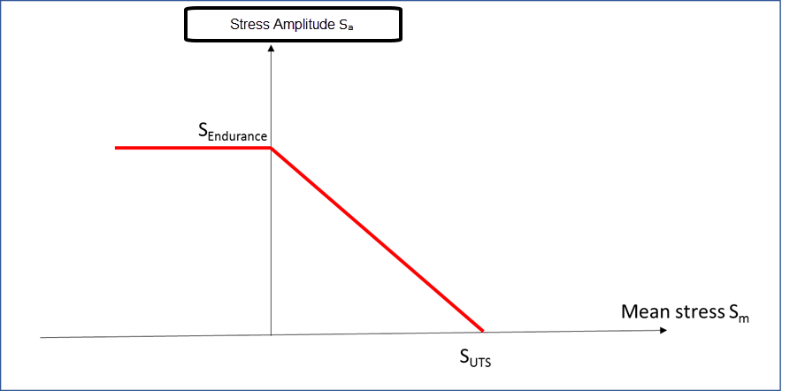
The Goodman method treats positive mean stress correction in the way that mean stress always accelerates fatigue failure, while it ignores the negative mean stress. This method gives conservative result for compressive mean stress.

A Haigh diagram characterizes different combinations of stress amplitude and mean stress for a given number of cycles to failure.

Findley Model

The Findley criterion is often applied for the case of finite long-life fatigue. The equation for each plane is as follows:

\frac{Δ τ}{2} + k σ_{n} = τ_{f}^{*} {(N_{f})}^{b}

Where:

τ_{f}^{*}

is computed from the shear fatigue strength coefficient,

τ_{f}^{'}

, using:

τ_{f}^{*} = \sqrt{1 + k^{2}} τ_{f}^{'}

The correction factor

\sqrt{1 + k^{2}}

typically has a set value of about 1.04.

Note:

τ_{f}^{*}

must be defined based on amplitude. If

τ_{f}^{'}

is not defined by the user, SimSolid calculates it using the following equation:

(30)

\begin{array}{l} τ_{f}^{'} = C f * 0.5 * S R I 1 \\ Where, \\ C f = \frac{2}{1 + \frac{k}{\sqrt{1 + k^{2}}}} \end{array}

The constant k is determined experimentally by performing fatigue tests involving two or more stress states. For ductile materials, k typically varies between 0.2 and 0.3.

FKM

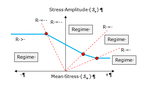
Based on FKM-Guidelines, the Haigh diagram is divided into four regimes based on the Stress ratio (R=S_min/S_max) values. The Corrected value is then used to choose the SN curve for the damage and life calculation stage.

The FKM equations below illustrate the calculation of Corrected Stress Amplitude ( $S_{e}^{A}$ ). The actual value of stress used in the Damage calculations is the Corrected stress Amplitude (which is $2 \cdot S_{e}^{A}$ ). These equations apply for SN curves that you input.

Regime 1 (R>1.0): $S_{e}^{A} = S_{a} (1 - M)$

Regime 2 (-∞≤R≤0.0): $S_{e}^{A} = S_{a} + M * S_{m}$

Regime 3 (0.0<R<0.5): $S_{e}^{A} = (1 + M) \frac{S_{a} + (\frac{M}{3}) S_{m}}{1 + \frac{M}{3}}$

Regime 4 (R≥0.5): $S_{e}^{A} = \frac{3 S_{a} {(1 + M)}^{2}}{3 + M}$

Where

S_{e}^{A}

is the stress amplitude after mean stress correction (Endurance stress),

S_{m}

is the mean stress,

S_{a}

is the stress amplitude, and M is the mean stress sensitivity.

Morrow

Morrow is the first to consider the effect of mean stress through introducing the mean stress $σ_{0}$ in fatigue strength coefficient by:

ε_{a}^{e} = \frac{(σ'_{f} - σ_{0})}{E} {(2 N_{f})}^{b}

Thus the entire fatigue life formula becomes:

ε_{a} = \frac{(σ_{f}^{'} - σ_{0})}{E} {(2 N_{f})}^{b} + ε_{f}^{'} {(2 N_{f})}^{c}

Morrow's equation is consistent with the observation that mean stress effects are significant at low value of plastic strain and of little effect at high plastic strain.

MORROW2 : Improves the Morrow method by ignoring the effect of negative mean stress.

Smith, Watson, and Topper

Smith, Watson, and Topper proposed a different method to account for the effect of mean stress by considering the maximum stress during one cycle (for convenience, this method is called SWT in the following). In this case, the damage parameter is modified as the product of the maximum stress and strain amplitude in one cycle.

ε_{a}^{S W T} σ_{\max} = ε_{a} σ_{a} = σ_{a} (\frac{σ'_{f}}{E} {(2 N_{f})}^{b} + ε'_{f} {(2 N_{f})}^{c})

The SWT method will predict that no damage will occur when the maximum stress is zero or negative, which is not consistent with reality.

When comparing the two methods, the SWT method predicted conservative life for loads predominantly tensile, whereas, the Morrow approach provides more realistic results when the load is predominantly compressive.

Fatemi-Socie

This model is for shear crack growth. During shear loading, the irregularly shaped crack surface results in frictional forces that will reduce crack tip stresses, thus hindering crack growth and increasing the fatigue life. Tensile stresses and strains will separate the crack surfaces and reduce frictional forces. Fractographic evidence for this behavior has been obtained. Fractographs from objects that have failed by pure torsion show extensive rubbing and are relatively featureless in contrast to tension test fractographs where individual slip bands are observed on the fracture surface.

To demonstrate the effect of maximum stress, tests with the six tension-torsion loading histories were conducted. They were designed to have the same maximum shear strain amplitudes. The cyclic normal strain is also constant for the six loading histories. The experiments resulted in nearly the same maximum shear strain amplitudes, equivalent stress and strain amplitudes and plastic work. The major difference between the loading histories is the normal stress across the plane of maximum shear strain.

The loading history and normal stress are shown in the figure at the top of each crack growth curve. Higher maximum stresses lead to faster growth rates and lower fatigue lives. The maximum stress has a lesser influence on the initiation of a crack if crack initiation is defined on the order of 10 mm, which is the size of the smaller grains in this material.

These observations lead to the following model that may be interpreted as the cyclic shear strain modified by the normal stress to include the crack closure effects.

\frac{Δ γ}{2} (1 + k \frac{σ_{n, \max}}{σ_{y}}) = \frac{τ_{f}^{'}}{G} {(2 N_{f})}^{b_{γ}} + γ_{f}^{'} {(2 N_{f})}^{c_{γ}}

The sensitivity of a material to normal stress is reflected in the value $k / σ y$ . Where, $σ y$ is stress where a significant total strain of 0.002 is used in SimSolid. If test data from multiple stress states is not available, k = 0.3. This model not only explains the difference between tension and torsion loading but also can be used to describe mean stress and non-proportional hardening effects. Critical plane models that include only strain terms cannot reflect the effect of mean stress or strain path dependent on hardening.

The transition fatigue life, 2N_t, is selected because the elastic and plastic strains contribute equally to the fatigue damage. You can obtain it from the uniaxial fatigue constants.

2 N_{f} = {(\frac{E ε_{f}^{'}}{σ_{f}^{'}})}^{(\frac{1}{b - c})}

Employ the Fatemi-Socie model to determine the shear strain constants.

\frac{Δ γ}{2} (1 + k \frac{σ_{n, \max}}{σ_{y}}) = \frac{τ_{f}^{'}}{G} {(2 N_{f})}^{b_{γ}} + γ_{f}^{'} {(2 N_{f})}^{c_{γ}}

First, note the exponents should be the same for shear and tension.

\begin{array}{l} b_{γ} = b \\ c_{γ} = c \end{array}

Shear modulus is directly computed from the tensile modulus.

G = \frac{E}{2 (1 + ν)}

You can estimate yield strength from the uniaxial cyclic stress strain curve.

σ_{y} = K^{'} {(0.002)}^{n^{'}} = \frac{σ_{f}^{'}}{ε_{f}^{' \frac{b}{c}}} {(0.002)}^{\frac{b}{c}}

Normal stresses and strains are computed from the transition fatigue life and uniaxial properties.

\frac{Δ ε_{p}}{2} = ε_{f}^{'} {(2 N_{t})}^{c}

\frac{Δ ε_{e}}{2} = \frac{σ_{f}^{'}}{E} {(2 N_{t})}^{b}

σ_{n, \max} = \frac{Δ σ}{4} = \frac{E Δ ε_{e}}{4}

Substituting the appropriate the value of elastic and plastic Poisson’s ratio gives:

\begin{array}{l} \frac{Δ γ_{e}}{2} = 1.3 \frac{Δ ε_{e}}{2} \\ \frac{Δ γ_{p}}{2} = 1.5 \frac{Δ ε_{p}}{2} \end{array}

Separating the elastic and plastic parts of the total strain results in these expressions for the shear strain life constants:

\begin{array}{l} τ_{f}^{'} = \frac{1.3 Δ ε_{e}}{2} (1 + k \frac{σ_{n, \max}}{σ_{y}}) \frac{G}{{(2 N_{t})}^{b_{γ}}} \\ γ_{f}^{'} = \frac{1.5 Δ ε_{p}}{2} (1 + k \frac{σ_{n, \max}}{σ_{y}}) \frac{G}{{(2 N_{t})}^{c_{γ}}} \end{array}

Brown-Miller

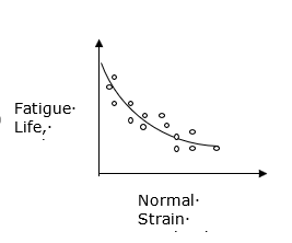
This model is for shear crack growth. Brown and Miller conducted combined tension and torsion tests with a constant shear strain range. The normal strain range on the plane of maximum shear strain will change with the ratio of applied tension and torsion strains. Based on the data shown below for a constant shear strain amplitude, Brown and Miller concluded that two strain parameters are needed to describe the fatigue process because the combined action of shear and normal strain reduces fatigue life.

Figure 4. Fatigue Life versus Normal Strain Amplitude

Influence of Normal Strain Amplitude

Analogous to the shear and normal stress proposed by Findley for high cycle fatigue, they proposed that both the cyclic shear and normal strain on the plane of maximum shear must be considered. Cyclic shear strains will help to nucleate cracks and the normal strain will assist in their growth. They proposed a simple formulation of the theory:

\frac{Δ \hat{γ}}{2} = \frac{Δ γ_{\max}}{2} + S Δ ε_{n}

Where $Δ \hat{γ}$

is the equivalent shear strain range and S is a material dependent parameter that represents the influence of the normal strain on material microcrack growth and is determined by correlating axial and torsion data. Here,

Δ γ_{\max}

is taken as the maximum shear strain range and

Δ ε_{n}

is the normal strain range on the plane experiencing the shear strain range

Δ γ_{\max}

. Considering elastic and plastic strains separately with the appropriate values of Poisson's ratio results in:

\frac{Δ γ_{\max}}{2} + S Δ ε_{n} = A \frac{σ_{f}^{'}}{E} {(2 N_{f})}^{b} + B ε_{f}^{'} {(2 N_{f})}^{c}

Where:

A = 1.3+0.7S

B = 1.5+0.5S

Mean stress effects are included using Morrow's mean stress approach of subtracting the mean stress from the fatigue strength coefficient. The mean stress on the maximum shear strain amplitude plane, $σ_{n}$ , is one half of the axial mean stress leading to:

\frac{Δ γ_{\max}}{2} + S Δ ε_{n} = A \frac{σ_{f}^{'} - 2 σ_{n, m e a n}}{E} {(2 N_{f})}^{b} + B ε_{f}^{'} {(2 N_{f})}^{c}