
/MAT/LAW24 (CONC)
Block Format Keyword This material law models brittle elastic-plastic behavior of concrete. A yield surface is deduced from an Ottosen triaxial failure surface. Orthotropic damage is modeled and cracks can open and close.
An optional embedded model allows to take into account steel rebars into a homogenized model. Otherwise, rebars are usually meshed with 1D or 3D elements.
This material law is compatible with solid elements only.
Format
| (1) | (2) | (3) | (4) | (5) | (6) | (7) | (8) | (9) | (10) |
|---|---|---|---|---|---|---|---|---|---|
| /MAT/LAW24/mat_ID/unit_ID or /MAT/CONC/mat_ID/unit_ID | |||||||||
| mat_title | |||||||||
| Ec | Icap | ||||||||
| fc | ft/fc | fb/fc | f2/fc | s0/fc | |||||
| Ht | Dsup | ||||||||
| ky | Hbp | Etc | |||||||
| vmax | |||||||||
| fk | f0 | Hv0 | Eps0 | hfac | |||||
| E | Et | ||||||||
Definition
| Field | Contents | SI Unit Example |
|---|---|---|
| mat_ID | Material identifier. (Integer, maximum 10 digits) |
|
| unit_ID | Unit identifier. (Integer, maximum 10 digits) |
|
| mat_title | Material title. (Character, maximum 100 characters) |
|
| Initial density. (Real) |
||
| Ec | Concrete elasticity Young's
modulus. (Real) |
|
| Poisson's ratio. (Real) |
||
| Icap | Cap
formulation flag. 8
(Integer) |
|
| fc | Concrete uniaxial compression
strength. (Real) |
|
| ft/fc | Concrete tensile strength ratio. Default = 0.10 (Real) |
|
| fb/fc | Concrete biaxial strength ratio. Default = 1.20 (Real) |
|
| f2/fc | Concrete confined strength ratio. Default = 4.00, if Icap = 0 or 1 Default = 7.00 if Icap = 2 (Real) |
|
| s0/fc | Concrete confining stress ratio. Default = 1.25 (Real) |
|
| Ht | Concrete tensile tangent modulus. Default = -Ec (Real) |
|
| Dsup | Concrete maximum damage. Default = 0.99999 (Real) |
|
| Concrete data total failure strain. Default = 1020 (Real) |
||
| ky | Concrete plasticity initial value of hardening
parameter (first part). Default = 0.5 (Real) |
|
| Concrete plasticity failure/plastic transition
pressure (first part). Default = 0.0 (Real) |
||
| Concrete plasticity proportional yield transition
pressure (first part). Default = -fc/3 (Real) |
||
| Hbp | Concrete plasticity base plastic modulus (first
part). 3 Default is computed by Starter (Real) |
|
| Etc | Concrete plastic modulus. 3
(Real) |
|
| Concrete plasticity dilatancy factor at yield
(second part). Default = -0.2, if Icap= 0 or 2 Default = 0.0, if Icap= 1 (Real) |
||
| Concrete plasticity dilatancy factor at failure
(second part). Default = 0.0 (Real) |
||
| vmax | Concrete plasticity maximum volumetric compaction
( < 0 ) (second part). Default = -0.35 (Real) |
|
| fk | Initial beginning of cap. 7 Default = -fc/3 (Real) |
|
| f0 | Initial end of cap. 7 Default = -0.8 fc, if Icap = 0 or 1 Default = -2 fc, if Icap = 2 (Real) |
|
| Hv0 | Initial triaxial plastic modulus. Default = 0.2 Ec (Real) |
|
| Eps0 | Reference plastic strain for plastic hardening
(Icap
= 2 only). Default = 0.02 (Real) |
|
| hfac | Reduction factor for plastic hardening default
(Icap
= 2 only). Default = 0.1 (Real) |
|
| E | Steel properties Young's
modulus. (Real) |
|
| Yield strength. (Real) |
||
| Et | Tangent modulus. (Real) |
|
| Rebar section fraction of reinforcement in
direction 1. (Real) |
||
| Rebar section fraction of reinforcement in
direction 2. (Real) |
||
| Rebar section fraction of reinforcement in
direction 3. (Real) |
Example (Concrete)
#RADIOSS STARTER
/UNIT/1
unit for mat
                   g                  mm                  ms
#---1----|----2----|----3----|----4----|----5----|----6----|----7----|----8----|----9----|---10----|
#-  2. MATERIALS:
#---1----|----2----|----3----|----4----|----5----|----6----|----7----|----8----|----9----|---10----|
/MAT/CONC/1/1
concrete - air dry
#              RHO_I
               .0024
#                E_c                  NU      Icap
               41200                  .2         0
#                 fc            ft_on_fc            fb_on_fc            f2_on_fc            s0_on_fc
                  44                   0                   0                   0                   0
#                H_t               D_sup             EPS_max
                   0                   0                   0
#                k_y                 r_t                 r_c                H_bp
                   0                   0                   0                   0
#            ALPHA_y             ALPHA_F               V_max
                -0.2                -0.1                   0
#                f_k                 f_0                H_v0                eps0               h_fac
                   0                   0                   0
#                  E             sigma_y                 E_t
                   0                   0                   0
#             ALPHA1              ALPHA2              ALPHA3
                   0                   0                   0
#---1----|----2----|----3----|----4----|----5----|----6----|----7----|----8----|----9----|---10----|
#ENDDATA
/END
#---1----|----2----|----3----|----4----|----5----|----6----|----7----|----8----|----9----|---10----|
Comments
- This material law can be used with only four parameters: and . Values are input as ratios of and are based on the failure of a typical concrete material.
- The parameters for the damage model
are:
Figure 1. Stress Strain Curve for LAW24 Damage Model. meridians of failure and yield surfaces 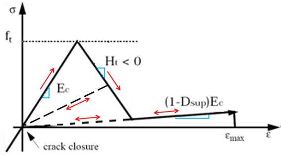
Where, is the uniaxial compression strength.
- The default value of the plastic modulus
in compression is defined as:The base plastic modulus is then calculated:
Figure 2. 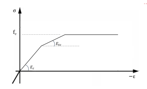
- The yield envelope is derived from the
failure envelope using a scale factor
.
-
is the hardening
parameter, it characterizes the limit of the
current elastic domain. The initial limit of the
elastic domain is set at
and the initial
failure surface at
.
The scale factor models the hardening effect depending on the mean stress .
In tension (when ), and the yield envelope and failure envelope are superimposed.
In compression (when ), the scale factor depends on Icap value (0, 1 or 2).Figure 3. Scale factor shapes the yield surface from the failure surface 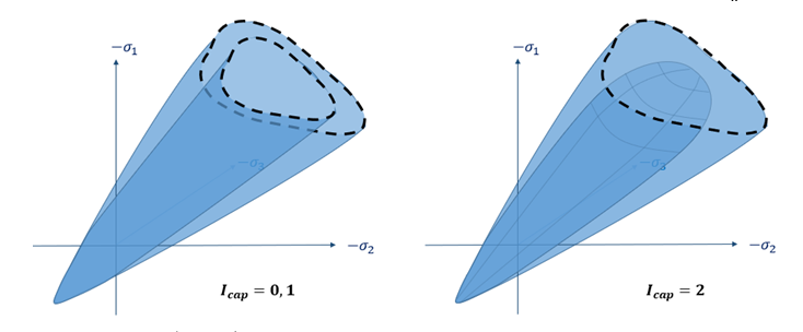
- For
Icap
=0 or 1:
Figure 4. 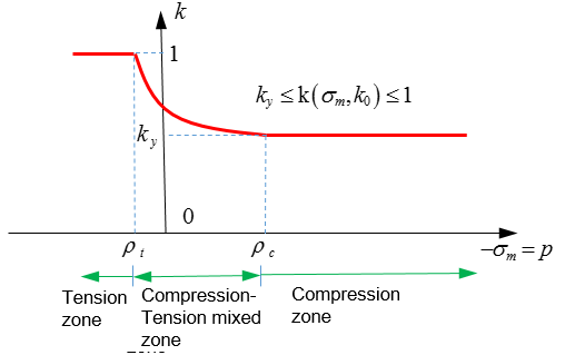
- For
Icap
=2 (with cap):
Figure 5. 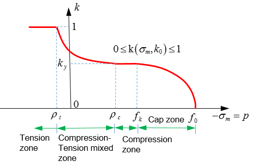
Where, and is mean stress (pressure), and are the first and second stress invariant. The factor can be output in time history file under VK keyword.
- For
Icap
=0 or 1:
- There is no cap effect when because there is no compaction. The default values of dilatancy parameters and were modified for Icap = 0 or 2 in Radioss 2017. These parameters should be negative with recommended values of -0.2 and -0.1, respectively. The default cap formulation was updated in Radioss 2017. To enable the original cap formulation used in Radioss 14.0 and older, set Icap = 1. The Icap =2 formulation is more accurate for triaxial and hydrostatic loadings. The cap hardening is a function of the compaction coefficient. The shear hardening modulus is reduced in the transition region which assures better stability. Icap = 2 must be used to output plastic strain using /ANIM/BRICK/EPSP or /H3D/SOLID/EPSP.
- The embedded rebar model is optional. It
uses an elastic-plastic with hardening material
model. When defining rebar section fractions, a
homogenized behavior is assumed for each element.
The element should be large enough to stand for a
Representative Elementary Volume (REV). This
homogenized model is mostly used with large
structures and a coarse mesh. Otherwise, rebar can
be modeled with trusses, springs, beams, or even
brick elements. the section ratio of rebars must
be provided
,
, and
:
Figure 6. 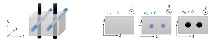
- The rebar directions must be defined in the orthotropic solid property /PROP/TYPE6. Otherwise, the local element coordinate r, s, and t are taken respectively as directions 1, 2, and 3; unless Isolid = 1 or 2 is used with Iframe = 2; in which case the orthotropic directions 1, 2 and 3 are defined with the local co-rotating element coordinate r, s, and t, when time = 0.
- In an axisymmetrical analysis, direction 3 is the direction.
- The 10 node tetrahedron elements are compatible with this law.