In Radioss these materials can be used to represent rock
or concrete materials.
These materials use a Drucker–Prager yield criterion1, which is a pressure-dependent model for determining whether
a material has failed or undergone plastic yielding.
Concrete Material (/MAT/LAW10 and /MAT/LAW21)
Drucker-Prager Yield Criteria
The material has failed or undergone plastic yielding is determined by pressure
using:
Where,
Second stress invariant (von Mises stress) of the deviatoric part of the
stress and .
First stress invariant (hydrostatic pressure).
In a uniaxial test.
Figure 1. Drucker-Prager yield criteria
A polynomial equation is used to describe the pressure at the Drucker-Prager yield surface of the material:
The constants of the polynomial are determined by:
If , the material is under yield surface and is
in the elastic region.
If , and the material is at the yield
surface.
If , and the material is past the yield surface
and has failed.
If , , which is the von Mises criterion.Figure 2.
Pressure Computation
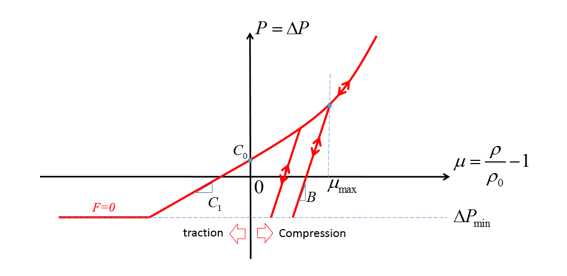
In LAW10, a polynomial equation with input parameters is used to describe the pressure. The pressure can
be plotted as a function of volumetric strain.
If , the pressure is and the pressure limit is .Figure 3. Pressure curve without external pressure
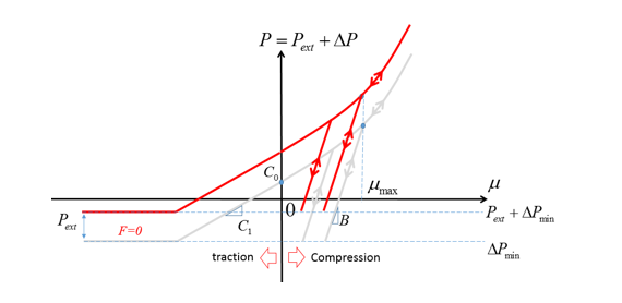
If , the pressure is shifted by , then and the pressure limit is .Figure 4. Pressure curve with external pressure
Here,
In traction or tension
the pressure is linear and limited by .
In compression the
pressure is nonlinear also limited by .
The only difference between the material laws is that in LAW10 the material constants are used to describe the pressure versus volumetric
strain ( curve). In LAW21 you can describe this curve via
function input fct_IDf.
Load and Unload
In LAW10 and LAW21 different loading and unloading paths of the curve can be considered by using the parameters
and B.
In Tension ()
For LAW10,
linear loading and unloading with (Figure 3).
For LAW21,
loading is defined using the input function
fct_IDf and
linear unloading with .
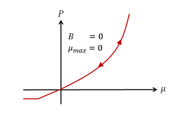
In Compression (), for both LAW10 and LAW21:
If neither B and
are defined, the loading and unloading path
are identical. Figure 5. Identical loading and unloading for LAW10 and
LAW21
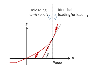
If either B or
is defined:
If only
B is defined, is the volumetric strain where the
tangent of curve is equal to B with .
If only
is defined, then B is the tangent
of curve at
. The loading and unloading in
compression is:
If , loading and unloading
path are identical.
If , loading and unloading
path are different, it is linear unloading with
slope B. Figure 6. Different loading and unloading
treatment for LAW10 and LAW21
Concrete Material (/MAT/LAW24)
LAW24 uses a Drucker-Prager criteria with or without a cap in yield to model a
reinforced concrete material. This material law assumes that the two failure mechanisms of
the concrete material are tensile cracking and compressive crushing.
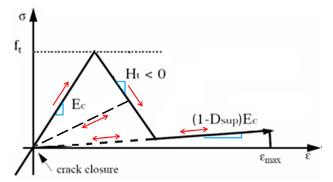
Concrete Tensile Behavior
In LAW24, the options Ht,
Dsup, and
can be used to describe tensile cracking and failure in
tension.Figure 7. LAW24 Tensile Loading
In the initial very small elastic phase, the material has an elastic modulus
Ec.
Once tensile strength, ft is
reached, the concrete starts to soften with the slope
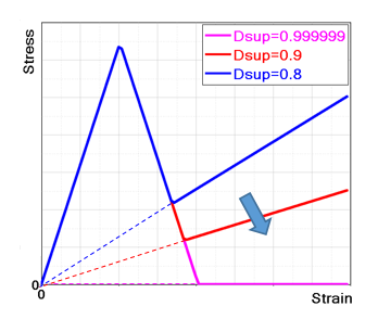
Ht. The maximum damage
factor, Dsup, is significant
because it enables the modeling of residual stiffness during and after a crack.Figure 8. Maximum Damage Factor Effects
The residual stiffness is computed as:
When there is crack closure, the concrete becomes elastic again, and the damage
factor (for each direction) is conserved.
The bearing capacity of concrete in tensile is much lower than in compression. It is
normally considered elastic when in tension.
It is recommended to choose a Dsup
value close to 1 (default is 0.99999) in order to minimize the current stiffness at
the end of the damage and consequently avoid residual stress in tension, which can
become very high if the element is highly deformed due to tension. This will happen
if the force causing the damage remains.
You can adjust the Dsup (and
Ht) in order to simulate and
fit the behavior of concrete reinforced by fibers. The concrete material fails once
it reaches the total failure strain .
Concrete Yield Surface in Compression
For concrete, the yield surface is the beginning of the plastic hardening zone which
is between the failure surface, , and the yield surface.
The yield surface is assumed to be the same as the failure surface in the tension
zone. In compression, the yield surface is a scaled down failure surface using the
factor . The yield in LAW24 for concrete is:
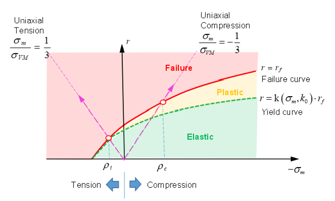
For Icap
=0 or 1 (without a cap in yield), the
yield curve is:Figure 9. Drucker-Prager Criteria without a Cap in
Yield
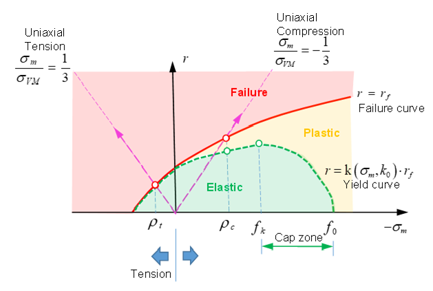
For Icap
=2 (with cap in yield), the yield is:Figure 10. Drucker-Prager Criteria with Cap in Yield
The material is above yield and below the failure surface which
is the plastic hardening phase.
The input parameter is the hydrostatic failure pressure in a uniaxial
tension test and is the hydrostatic pressure by failure in a uniaxial
compression test.
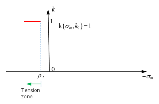
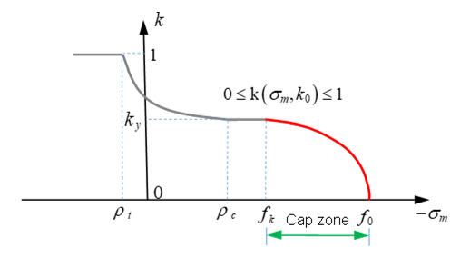
The scale factor is a function of mean stress and can be described as:
When (in tension) the scale factor . In this case, the yield surface equals the
failure surface, .Figure 11. Function in the Tension Zone
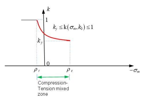
In the tension-compression region, , then
with Figure 12. Function in the
Compression-Tension Mixed Zone
The rest of the curve depends on the
Icap option and the
different scale factors used.
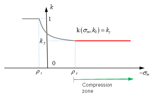
For Icap
=0 or 1 and (in compression), then Figure 13. Function in the Compression
Zone
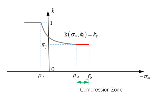
For Icap
=2 (with cap in yield) and (in compression), then Figure 14. Function in Drucker-Prager
Criteria without a Cap
In (in cap zone)
with Figure 15. Function in
Drucker-Prager Criteria with a Cap
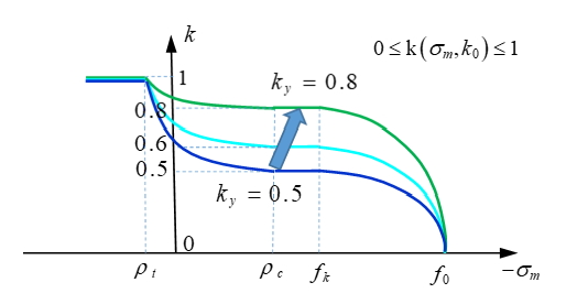
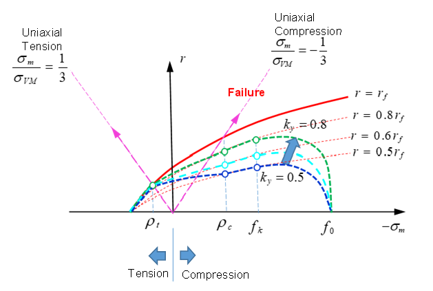
The material constant should be . A higher value of results in a higher yield surface.
For example, if Icap
=2 (yield with cap), the difference of yield surface between and (Figure 16). The default value of in LAW24 is 0.5.Figure 16. Affect of Different Function Values Figure 17. Drucker-Prager Criteria with Different Function Values
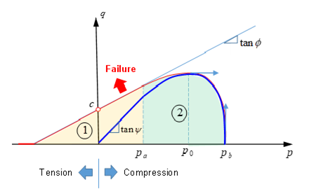
Concrete Plastic Flow Rule in Compression
A non-associated plastic flow rule is used in LAW24. The plastic flow rule
is:
Where,
Plastic dilatancy.
Governs the volumetric plastic flow.
First stress invariant (hydrostatic pressure).
Experimentally, is a linear function of :
If , then which means the material is in yield.
If , then becomes negative is the cap region.
If , then which means the material has failed.
The values of are used to describe the material beyond yield, but
before failure. It is recommended to use -0.2 and -0.1 for in LAW24. If very small values of are used, there is no volumetric plasticity (no cap
region).
Concrete Crushing Failure in Compression
Failure surface is given by:
Where, , and is Lode angle, such as:
An Ottosen surface is built to design this surface using:
Where, , , and are
4 values which shape the surface and
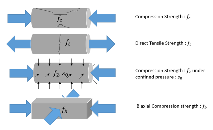
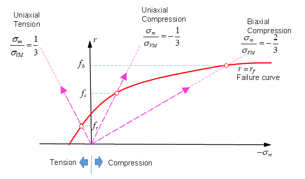
For concrete, the compression failure curve can be defined with a strength of:
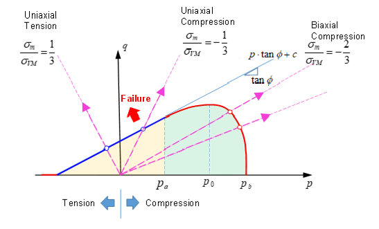
Uniaxial tension (triaxiality is 1/3)
Uniaxial compression (triaxiality is -1/3)
Biaxial compression (triaxiality is -2/3)
Confined compression strength (tri-axial test)
Under confined pressure
The best way to fully determine the 3D failure envelope is to get experimental data
for all of these values, which are schematically illustrated in Figure 18.Figure 18. Failure Parameters that Fully Determine 3D Failure
Envelope
Table 1. Input from the 4 Experimental Tests
Load Type
Surface Point
Default Input
Criteria
Pressure
Lode Angle
Compression
Mandatory
Direct Tensile
Biaxial Compression
If
Icap =
1
If Icap = 2
Compression Strength under Confinement
Pressure
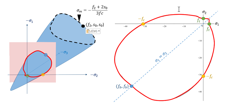
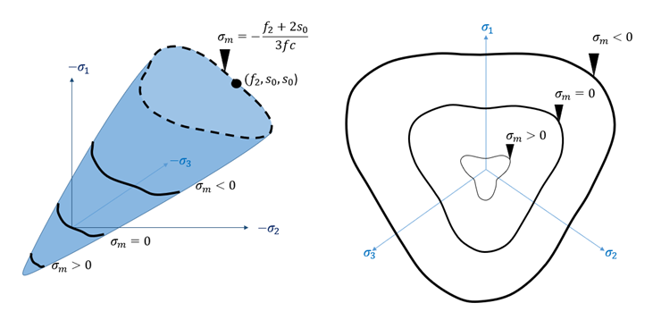
Figure 19 and Figure 20 show the points that determine the failure surface.Figure 19. Trace of failure surface with planar stress plane Figure 20. Failure trace with several cut plan which are normal to the
hydrostatic axis
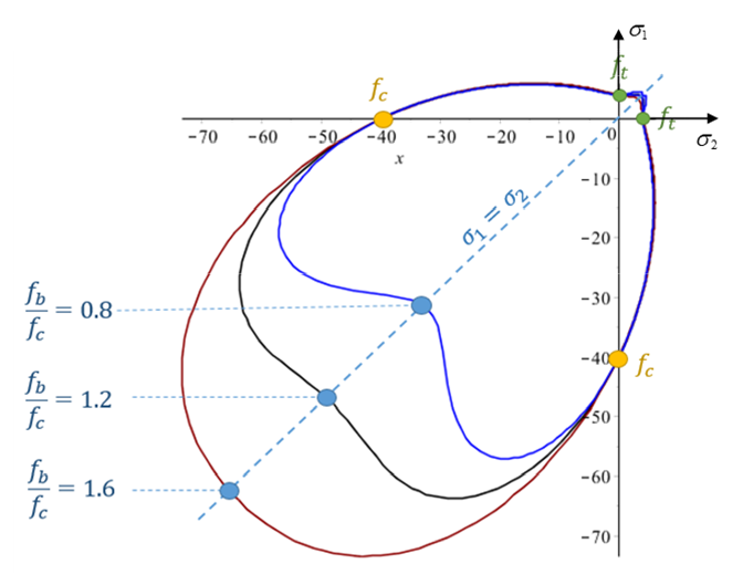
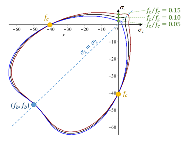
From these plots that the failure envelope is not a convex surface. Figure 21 shows this behavior.Figure 21. Influence of the biaxial compressive strength value with all
other characteristic failure points fixed Figure 22. Influence of the compressive strength value with all other
characteristic failure points fixed Figure 23. Influence of the tensile strength value with all other
characteristic failure points fixed
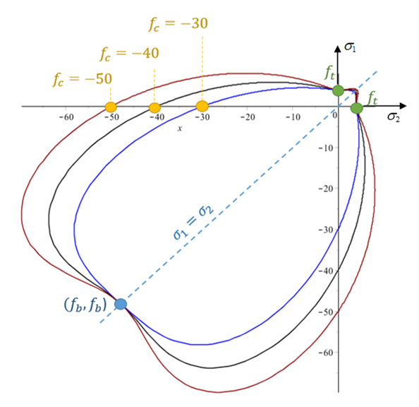
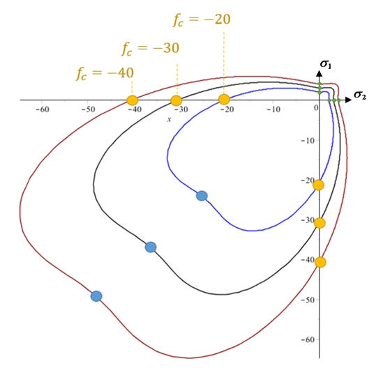
In this particular case, the compressive strength is changing but all other ratios
are fixed . This leads to an envelope scaling, as shown in
Figure 24.Figure 24. Influence of compressive strength value. All other ratios are fixed.
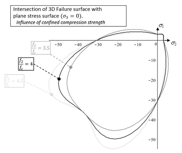
Here with same strength in LAW24, but different confined compression strength
.Figure 25. Failure envelope on the plane stress surface influenced by
the triaxial failure point
and the ratios in the space (used to define the concrete failure) are:Figure 26. Different tests (uniaxial tension, uniaxial compression, and
biaxial compression) to determine failure curve
Where the failure curve is defined using and is the mean stress (pressure), then and are the first and second stress invariants.
The material fails once it reaches the failure curve
.
Concrete
Reinforcement
In Radioss there are two
different ways to simulate the reinforcement in concrete.
One way is to use beam or truss elements and connect them to the concrete
with kinematic conditions.
Another way is to use the parameters in LAW24 along with the orthotropic
solid property /PROP/TYPE6 to define the reinforced
direction. Parameters in LAW24 are used to define the
reinforcement cross-section area ratio to the whole concrete section area in
direction 1, 2, 3.
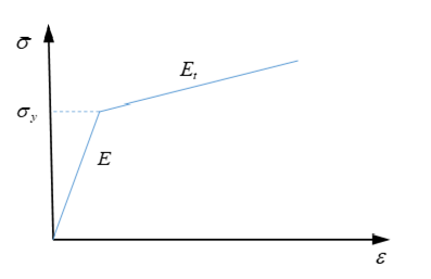
Where, is the yield stress of the reinforcement. If steel
is used as a reinforcement, then is the yield stress of steel and is the modulus of steel in the plastic phase.Figure 27. Stress-Strain Curve of Reinforcement (steel)
Concrete Material (/MAT/LAW81)
LAW81 can be used to model rock or concrete materials.
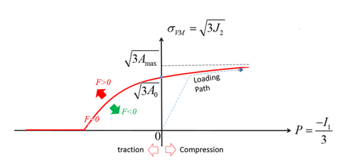
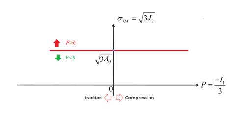
Drucker-Prager Yield Criteria
LAW81 uses a Drucker–Prager yield criterion where the yield surface and the failure
surface are the same. The yield criteria is:
Where,
von Mises stress with
Pressure is defined as
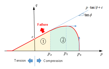
Figure 28. Yield Surface (LAW81)
The yield surface can be described in two parts:
The linear part (), where the scale function is which leads to the von Mises stress being
linearly proportional to pressure:
Where,
Cohesive and is the intercept of yield envelope with the
shear strength.
If , the material has no
strength under tension.
Angle of internal friction, which defines the slope of the
yield envelope.
and are also used to define the Mohr-Coulomb yield
surface. The Drucker-Prager yield surface is a smooth version of the
Mohr-Coulomb yield surface.
The second part () of the yield surface simulates a cap limit.
An increase of pressure in a rock or concrete material will increase the
yield of the material; but, if pressure increases enough, then the rock or
concrete material will be crushed. The Drucker-Prager model with the cap
limit can be used to model this behavior. The cap limit defined in part
and uses the scale
function:
The von Mises stress is:
Where,
Curve is defined using the
fct_IDPb
input
Computed by Radioss using the
input ratio value.
with .
Where, is the maximum point of yield curve,
where
If , then and the yield function is then,
which means the material is
crushed.
The input parameters need to determine for the Drucker–Prager yield
surface. At least four tests are needed to fit these parameters. In the simplest
case, uniaxial tension and uniaxial compression can be used to determine the linear
part, . To determine biaxial compression tests and
compression/compression tests are needed (refer to CC00 and CC01 in RD-V: 0250 Concrete Validation with Kupfer Tests).Figure 29. Yield Surface of LAW81 Showing Different Load
Conditions
For most materials such as metal, the plastic strain increment could be considered
normal to yield surface. However, if the plastic strain increment normal to yield
surface is used for rock or concrete materials, the plastic volume expansion is
overestimated. Therefore, a non-associated plastic flow rule is used in these
materials. In LAW81 the plastic flow function defined as:
if
if
if
Since the pressure is , the yield function and plastic flow function are the same and the following condition is
fulfilled:
The pressure can be calculated using the yield surface where . With defined as:
The parameter can be determined using the von Mises stress at pressure, in the function.Figure 30. Yield Surface of LAW81 with Plastic Flow
1 Han, D. J.,
and Wai-Fah Chen. "A nonuniform hardening plasticity model for concrete
materials." Mechanics of materials 4, no. 3-4 (1985):
283-302

 (
), where the scale function is
which leads to the von Mises stress being
linearly proportional to pressure:Where,
(
), where the scale function is
which leads to the von Mises stress being
linearly proportional to pressure:Where, (
) of the yield surface simulates a cap limit.
An increase of pressure in a rock or concrete material will increase the
yield of the material; but, if pressure increases enough, then the rock or
concrete material will be crushed. The Drucker-Prager model with the cap
limit can be used to model this behavior. The cap limit defined in part
(
) of the yield surface simulates a cap limit.
An increase of pressure in a rock or concrete material will increase the
yield of the material; but, if pressure increases enough, then the rock or
concrete material will be crushed. The Drucker-Prager model with the cap
limit can be used to model this behavior. The cap limit defined in part