
/MAT/LAW124 (CDPM2)
Block Format Keyword A concrete material law accounting for plasticity, damage, and strain rate effect.
Format
| (1) | (2) | (3) | (4) | (5) | (6) | (7) | (8) | (9) | (10) |
|---|---|---|---|---|---|---|---|---|---|
| /MAT/LAW124/mat_ID/unit_ID or /MAT/CDPM2/mat_ID/unit_ID | |||||||||
| mat_title | |||||||||
| E | IDEL | IRATE | FCUT | ||||||
| ECC | HP | ||||||||
| AH | BH | CH | DH | ||||||
| AS | BS | DF | DFLAG | DTYPE | IREG | ||||
| WF | WF1 | FT1 | EFC | ||||||
Definition
| Field | Contents | SI Unit Example |
|---|---|---|
| mat_ID | Material identifier. (Integer, maximum 10 digits) |
|
| unit_ID | (Optional) Unit identifier. (Integer, maximum 10 digits) |
|
| mat_title | Material title. (Character, maximum 100 characters) |
|
| Initial
density. (Real) |
||
| E | Young’s
modulus. (Real) |
|
| Poisson’s
ratio. (Real) |
||
| IDEL | Element deletion flag.
(Integer) |
|
| IRATE | Rate dependency flag.
(Integer) |
|
| FCUT | Strain rate filtering
frequency. Default = 10 kHz (Real) |
|
| ECC | Eccentricity. Default in Comment 6 (Real) |
|
| Initial hardening. Default = 0.3 (Real) |
||
| Strength limit in
tension. (Real) |
||
| Strength limit in
compression. (Real) |
||
| HP | Hardening
modulus. (Real) |
|
| AH | Compressive damage 1st
ductility parameter. Default = 0.08 (Real) |
|
| BH | Compressive damage 2nd
ductility parameter. Default = 0.003 (Real) |
|
| CH | Compressive damage 3rd
ductility parameter. Default = 2.0 (Real) |
|
| DH | Compressive damage 4th
ductility parameter. Default = 1.0E-6 (Real) |
|
| AS | First ductility measure
parameter.4 Default = 15.0 (Real) |
|
| BS | Second ductility measure
parameter. Default = 1.0 (Real) |
|
| DF | Dilation coefficient. Default = 0.85 (Real) |
|
| DFLAG | Damage model type.
(Integer) |
|
| DTYPE | Tensile damage shape.
(Integer) |
|
| IREG | Regularization flag.
(Integer) |
|
| WF | Tensile inelastic
displacement/strain at failure. Dimension depends on IREG parameter value. 4 7 (Real) |
|
| WF1 | Tensile in elastic
displacement/strain at softening slope change (bilinear damage
only). Dimension depends on IREG parameter value. 4 Default = 0.15*WF (Real) |
|
| FT1 | Tensile strength at
WF1. Default = 0.3*FT (Real) |
|
| EFC | Compressive inelastic strain close
to failure. 8 Default = 1.0E-4 (Real) |
Example
#RADIOSS STARTER
#---1----|----2----|----3----|----4----|----5----|----6----|----7----|----8----|----9----|---10----|
/UNIT/1
unit for mat
                  Mg                  mm                   s
#---1----|----2----|----3----|----4----|----5----|----6----|----7----|----8----|----9----|---10----|
/MAT/LAW124/1/1
Concrete CDPM2
#        Init. dens.
              2.3E-9
#                  E                  NU                IDEL               IRATE                FCUT
               28000                0.19                   1                   2                   0
#                ECC                 QH0                  FT                  FC                  HP
                   0                   0                 3.5                33.6                 0.5
#                 AH                  BH                  CH                  DH
                   0                   0                   0                   0
#                 AS                  BS                  DF               DFLAG     DTYPE      Ireg
                   0                   0                   0                   1         1         1
#                 WF                 WF1                 FT1                 EFC
               0.006                   0                   0              0.0005
#---1----|----2----|----3----|----4----|----5----|----6----|----7----|----8----|----9----|---10----|
#enddata
/END
#---1----|----2----|----3----|----4----|----5----|----6----|----7----|----8----|----9----|---10----|
Comments
- The CDPM2 material law is a user-friendly concrete material law,
which considers several phenomena. Only a few parameters are mandatory to
easily use this constitutive model. The mandatory physical parameters
are:
- Young’s modulus
- Poisson’s ration
- Tensile strength
- Compressive strength
- Tensile fracture energy
- (Optional) Compression fracture energy
- For this law, the elastic behavior is supposed to be isotropic. The
plastic behavior is then characterized by the following yield function
(Figure 1):
Where the Haigh-Westergaard coordinates in stresses space are considered:
, ,
Where,- Hardening variable
- Limit strength in compression
- Limit strength in tension
- A parameter considering the effect of eccentricity
Figure 1. CDPM2 model yield function shape (from Grassl) 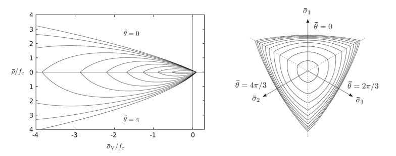
Then and are the two hardening functions defined with (Figure 2):Figure 2. Hardening functions shape (from Grassl) 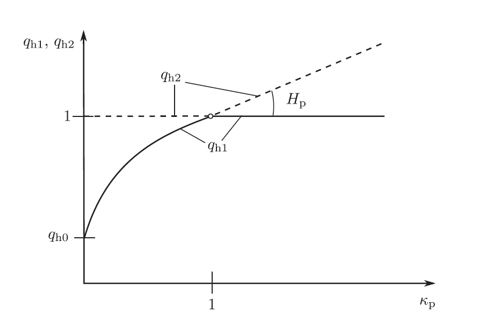
Here, is the initial hardening defined so that . is the hardening modulus whose recommended value is 0.5. The evolution of the internal variable is detailed below.
The William-Warnke function is used to develop the deviatoric section shape between tension and compression (Figure 1).
- The plastic strain evolution is defined by a non-associated plastic
potential using the following equation:
With
Where, is the dilation parameter.
This plastic potential is used to compute the evolution of the plastic strain tensor and, thus, the evolution of the internal variable as:
with
Where, is the Euclidian norm of the increment of the plastic strain tensor.
- The CDPM2 model
considers an unsymmetrical damage evolution between tension and compression.
These variables are respectively denoted by
and
. The damage variables evolution is triggered
by a strain criterion defined by:When this criterion is reached, the damage history variables to the corresponding loading case (tension or compression) are updated:
- In Tension:
, , and
- In
Compression:
, and
With,
, , with
The inelastic strains can be obtained from damage history variable using the following equations:
and
The damage history variable finally enables to update the corresponding damage variables.
Regarding tensile damage, three different evolution shapes are available depending on the DTYPE parameter value:- DTYPE = 1: Linear damage
where
is the strength limit at the
beginning of damage, and
is the failure displacement for
which the stiffness becomes null (Figure 3).
Figure 3. Uniaxial tension test on a single unit element using linear damage evolution . with =3.5 MPa and =0.002 mm 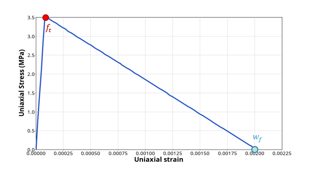
- DTYPE = 2: Bilinear damage
which is very similar to the linear damage apart from the use of
the couple of values
and
which define the coordinates of
the points where damage evolution changes its slope (Figure 4).
Figure 4. Uniaxial tension test on a single unit element using bilinear damage evolution . with =3.5 MPa, =1.5 MPa, =0.00075 mm and =0.002 mm 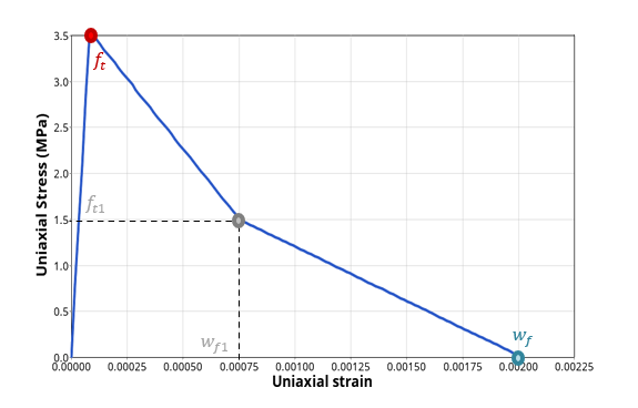
- DTYPE = 3: Exponential
damage where the displacement threshold
corresponds to the meeting point
between uniaxial strain axis, and tangent curve to the beginning
of stress softening (Figure 5).
Figure 5. Uniaxial tension test on a single unit element using exponential damage evolution . with =3.5 MPa and =0.002 mm 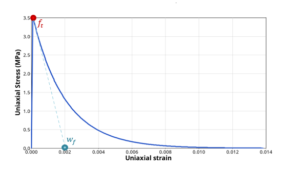
In these different equations, is a parameter that can be used to avoid mesh size dependency. When IREG = 1, no regularization method is used, and is set to 1. In that case, the critical value becomes a critical strain with no dimension. Otherwise, if IREG = 2, the Hillerborg’s regularization method 2 (also called Crack Brand method 3) is used, and equals the initial element size. Then, the critical value becomes a critical displacement homogeneous to a displacement. Hillerborg’s regularization method is to ensure that the tensile fracture energy denoted remains constant no matter what element size is used (Figure 6).Figure 6. Uniaxial tension test with bilinear damage on two different mesh sizes with IREQ = 0 (left); IREQ = 1 (right) 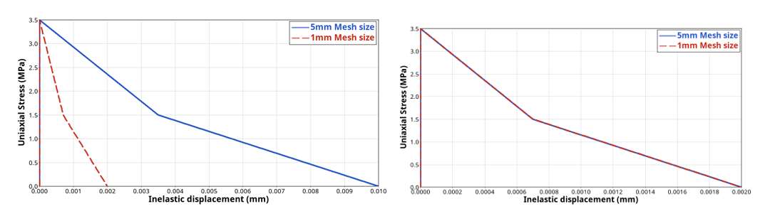
Regarding compression damage, only the exponential evolution shape is available without any regularization method (Figure 7). Mesh size dependency is assumed to be less sensitive.Figure 7. Uniaxial compression test on a single unit element . with 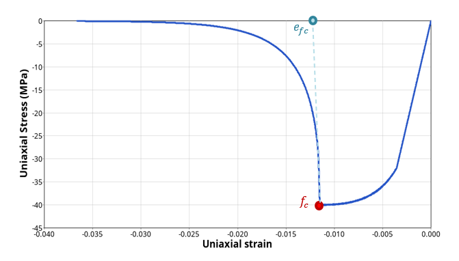
The effect of damage on stress computation will depend on the DFLAG parameter value:- DFLAG = 1: Non-symmetric
softening which considers the crack closure effect when
switching from tension to compression, recovering the initial
stiffness. On the opposite, a switch from tension to compression
re-opens the already existing cracks. (Figure 8).Where, and are respectively the tension and compression part of the undamaged (effective) stress tensor.
Figure 8. Loading/unloading uniaxial test with non-symmetrical damage softening 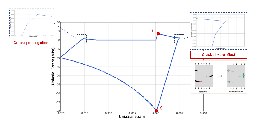
- DFLAG = 2: Isotropic
softening that considers only the effect of tensile damage in
both tension and compression. Then crack closure is not
considered. No changes of stiffness are observed when switching
from tension to compression or the opposite (Figure 9). Tensile damage is also
less likely to evolve in compression.
Figure 9. Loading/unloading uniaxial test with isotropic damage softening 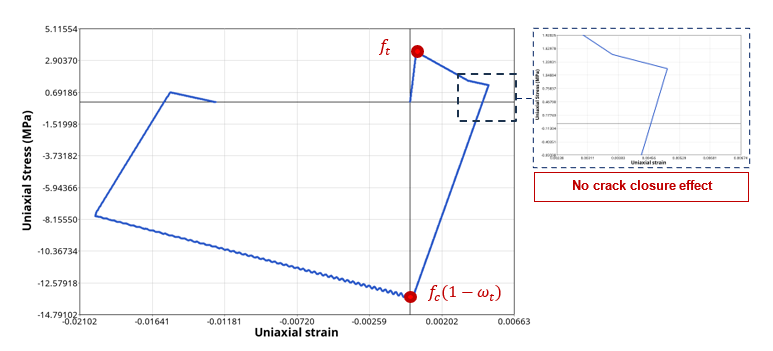
- DFLAG = 3: Multiplicative
softening where the effect of both tension and compression
damage are considered and cumulated on the behavior (Figure 10).
Figure 10. Loading/unloading uniaxial test with multiplicative damage softening 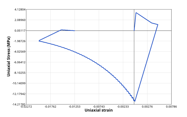
- In Tension:
- The last phenomena considered by CDPM2 model is the strain rate
dependency. At a high strain rate, the concrete is more likely to have a
larger tension or compression strength limit. This is introduced by the
following equations:
, and
The dynamic increase factor (DIF) is computed with:
Where, is the compression factor defined above in damage history variables equations in Comment 4.
There is then a different strain rate dependency between tension and compression as concrete is more sensitive to strain rate effect in tension than in compression. The two dynamic increased factor for both tension and compression are computed with:
with ,
with ,
The equivalent deviatoric strain rate is used to compute the DIF in the equations above.
No parameters need to be identified for strain rate effect. You only need to set the flag IRATE to 2. Figure 11 shows the expected tendency of strain rate effect on the CDPM2 behavior. By increasing the strength limits in tension/compression, the dissipated energy during failure is also affected which is often observed experimentally.Figure 11. Uniaxial tests in tension/compression with strain rate dependency (IRATE = 1) 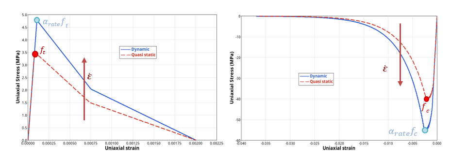
- Default value of
eccentricity can be obtained with:
and
- The tensile fracture
energy,
is not used directly as an input in the
model but is used to calculate the value of the tensile inelastic
displacement/strain at failure
.
For the linear softening law (DTYPE = 1), the tensile fracture energy is:
(if IREG = 2, default)
(if IREG = 1 with h= reference element size for identification)
For the bilinear softening law (DTYPE = 2), the tensile fracture energy is:
Suppose that = 0.3 and = 0.15, this leads to:
(if IREG = 2, default)
(if IREG = 1) with h = reference element size for identification)
- The compression
fracture energy,
is not used directly as an input in the
model but is used to calculate the value of the compressive inelastic strain
close to failure as:
with h= reference element size for identification and is the ductility measure:
- Global damage variable can be output using /ANIM/BRICK/DAMG or /H3D/SOLID/DAMG. Two modes of
damage can be plotted using MODE = I or
ALL:
- Mode 1: tension damage
- Mode 2: compression damage